Marker gene identification with COSG#

Setting basics#

[1]:

import numpy as np
import pandas as pd
import scanpy as sc
sc.set_figure_params(dpi=80,dpi_save=300, color_map='Spectral_r',facecolor='white')
from matplotlib import rcParams
# To modify the default figure size, use rcParams.
rcParams['figure.figsize'] = 4, 4
rcParams['font.sans-serif'] = "Arial"
rcParams['font.family'] = "Arial"
sc.settings.verbosity = 3
sc.logging.print_header()

scanpy==1.9.1 anndata==0.8.0 umap==0.5.3 numpy==1.21.6 scipy==1.7.3 pandas==1.4.4 scikit-learn==1.1.2 statsmodels==0.13.2 python-igraph==0.10.4 louvain==0.7.1 pynndescent==0.5.11

Setting colors#

[2]:

### Palette
scane_color=["#e6194b","#3cb44b","#ffe119",
"#4363d8","#f58231","#911eb4",
"#46f0f0","#f032e6","#bcf60c",
"#fabebe","#008080","#e6beff",
"#9a6324",
             "#800000",
"#aaffc3","#808000","#ffd8b1",
"#000075","#808080"
            ]
import seaborn as sns
self_palette2=sns.color_palette(np.hstack((scane_color,sc.pl.palettes.godsnot_102)))

# https://matplotlib.org/3.1.0/tutorials/colors/colormap-manipulation.html#sphx-glr-tutorials-colors-colormap-manipulation-py
# # https://gree2.github.io/python/2015/05/06/python-seaborn-tutorial-choosing-color-palettes
from matplotlib import cm
from matplotlib import colors, colorbar
cmap_own = cm.get_cmap('magma_r', 256)
newcolors = cmap_own(np.linspace(0,0.75 , 256))
Greys = cm.get_cmap('Greys_r', 256)
newcolors[:10, :] = Greys(np.linspace(0.8125, 0.8725, 10))
pos_cmap = colors.ListedColormap(newcolors)
di_cmap=sns.diverging_palette(138,359,s=72,l=50,sep=27,n=15,as_cmap=True)

Setting paths#

[3]:

save_dir='/n/scratch/users/m/mid166/Result/single-cell/Methods/COSG/COSG_tutorial'
sc.settings.figdir = save_dir
prefix='COSG_tutorial_SEA-AD'
import os
if not os.path.exists(save_dir):
    os.makedirs(save_dir)
sc.set_figure_params(dpi=80,dpi_save=300, color_map='viridis',facecolor='white')
rcParams['figure.figsize'] = 4, 4

Load the data#

The 20k subsampled snRNA-seq data from Allen SEA-AD project is available in google drive: https://drive.google.com/file/d/1nH-CRaTQFxJ5pAVpy8_hUQn1nrIcakq2/view?usp=drive_link.

The original data is available in https://portal.brain-map.org/explore/seattle-alzheimers-disease.

mkdir -p /n/scratch/users/m/mid166/Result/single-cell/Enhancer/SEA-AD/
cd /n/scratch/users/m/mid166/Result/single-cell/Enhancer/SEA-AD/
gdrive files download 1nH-CRaTQFxJ5pAVpy8_hUQn1nrIcakq2

[4]:

adata=sc.read('/n/scratch/users/m/mid166/Result/single-cell/Enhancer/SEA-AD/SEA-AD_RNA_MTG_subsample_excludeReference_20k_piaso.h5ad')

[5]:

adata.shape

[5]:

(20000, 36601)

[6]:

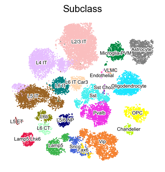
sc.pl.embedding(adata,
            basis='X_umap',
           color=['Subclass'],
           palette=self_palette2,
           legend_fontoutline=2,
           legend_fontweight=5,
           cmap='Spectral_r',
           ncols=3,
           size=10,
           frameon=False)

../_images/notebooks_24_COSG_tutorial_12_0.png

[7]:

sc.pl.embedding(adata,
    basis='X_umap',
    color=['Subclass'],
    palette=self_palette2,
    legend_fontoutline=2,
    legend_fontsize=7,
    legend_fontweight=5,
    legend_loc='on data',
    cmap='Spectral_r',
    ncols=3,
    size=10,
    frameon=False)

../_images/notebooks_24_COSG_tutorial_13_0.png

The data is normalized, and the raw UMI counts were saved in adata.layers['UMIs']:

[8]:

adata.X.data

[8]:

array([0.8813792 , 2.510722  , 0.8813792 , ..., 0.37347588, 0.37347588,
       1.1829159 ], dtype=float32)

Import COSG#

Install the latest version of COSG via pip install git+https://github.com/genecell/COSG.git from genecell/COSG:

[9]:

import cosg

[10]:

%%time
groupby='Subclass'
cosg.cosg(adata,
    key_added='cosg',
    # use_raw=False, layer='log1p', ## e.g., if you want to use the log1p layer in adata
    mu=100,
    expressed_pct=0.1,
    remove_lowly_expressed=True,
    n_genes_user=adata.n_vars, ### Use all the genes, to enable the calculation of transformed COSG scores
    # n_genes_user=100,
    groupby=groupby,
    return_by_group=True,
    verbosity=1
)

Finished identifying marker genes by COSG, and the results are in adata.uns['cosg'].
CPU times: user 7.79 s, sys: 3.12 s, total: 10.9 s
Wall time: 10.9 s

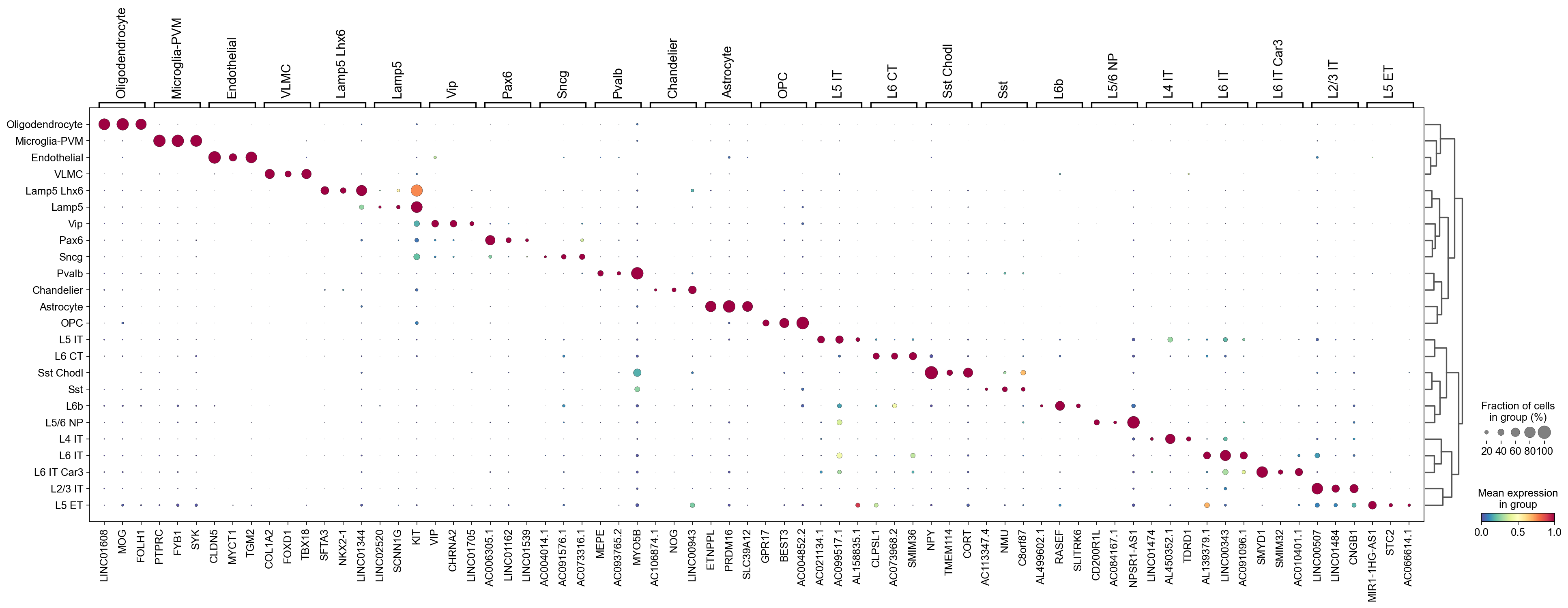
Let’s visualize the top marker genes identified by COSG with dotplot. There are two ways to build a dendrogram, one with use_rep and one using the category orders in adata.obs[groupby].

Here is the dotplot using the low-dimensional cell representations specified by use_rep:

[11]:

cosg.plotMarkerDotplot(
    adata,
    groupby='Subclass',
    top_n_genes=3,
    key_cosg='cosg',
    use_rep='X_scVI',
    swap_axes=False,
    standard_scale='var',
    cmap='Spectral_r',
    # save='test.pdf'
)

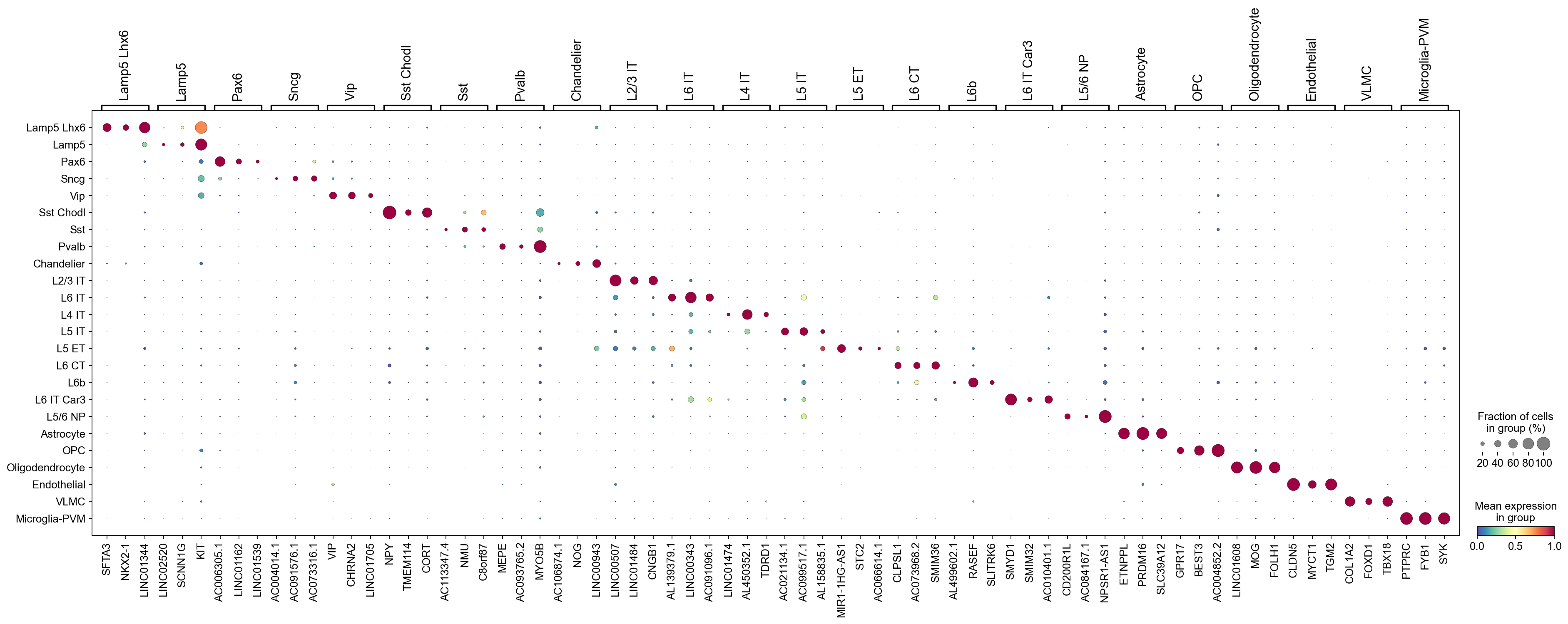
../_images/notebooks_24_COSG_tutorial_21_0.png

Use the category orders in adata.obs[groupby]:

[12]:

cosg.plotMarkerDotplot(
    adata,
    groupby='Subclass',
    top_n_genes=3,
    key_cosg='cosg',
    use_rep=None,
    swap_axes=False,
    standard_scale='var',
    cmap='Spectral_r',
    # save='test.pdf'
)

../_images/notebooks_24_COSG_tutorial_23_0.png

Check the top marker genes:

[13]:

pd.DataFrame(adata.uns['cosg']['names']).head()

[13]:

	Lamp5 Lhx6	Lamp5	Pax6	Sncg	Vip	Sst Chodl	Sst	Pvalb	Chandelier	L2/3 IT	...	L6 CT	L6b	L6 IT Car3	L5/6 NP	Astrocyte	OPC	Oligodendrocyte	Endothelial	VLMC	Microglia-PVM
0	SFTA3	LINC02520	AC006305.1	AC004014.1	VIP	NPY	AC113347.4	MEPE	AC106874.1	LINC00507	...	CLPSL1	AL499602.1	SMYD1	CD200R1L	ETNPPL	GPR17	LINC01608	CLDN5	COL1A2	PTPRC
1	NKX2-1	SCNN1G	LINC01162	AC091576.1	CHRNA2	TMEM114	NMU	AC093765.2	NOG	LINC01484	...	AC073968.2	RASEF	SMIM32	AC084167.1	PRDM16	BEST3	MOG	MYCT1	FOXD1	FYB1
2	LINC01344	KIT	LINC01539	AC073316.1	LINC01705	CORT	C8orf87	MYO5B	LINC00943	CNGB1	...	SMIM36	SLITRK6	AC010401.1	NPSR1-AS1	SLC39A12	AC004852.2	FOLH1	TGM2	TBX18	SYK
3	AL355482.1	AC099482.2	ABCB5	AL161629.1	AJ006995.1	GHRH	LINC02133	LRRC38	AC006065.4	AC008574.1	...	KL	SCUBE1	AC073225.1	LINC02042	OBI1-AS1	LINC01546	CD22	SRARP	C7	IKZF1
4	HCRTR2	CPLX3	LINC01416	AC004862.1	NPR3	DDC	OTOF	AC006364.1	SCUBE3	LINC02714	...	AC092114.1	FIBCD1	DCSTAMP	NPSR1	SLC14A1	VCAN-AS1	SLCO1A2	FENDRR	FMO2	PIK3R5

5 rows × 24 columns

Check the corrsponding COSG scores:

[14]:

pd.DataFrame(adata.uns['cosg']['scores']).head()

[14]:

	Lamp5 Lhx6	Lamp5	Pax6	Sncg	Vip	Sst Chodl	Sst	Pvalb	Chandelier	L2/3 IT	...	L6 CT	L6b	L6 IT Car3	L5/6 NP	Astrocyte	OPC	Oligodendrocyte	Endothelial	VLMC	Microglia-PVM
0	0.292173	0.058870	0.028365	0.068951	0.350845	0.381491	0.095953	0.362747	0.053039	0.527400	...	0.013717	0.105420	0.668806	0.431743	0.767967	0.450832	0.832948	0.801609	0.763216	0.871644
1	0.231243	0.019967	0.012673	0.068790	0.328894	0.053314	0.049051	0.172069	0.028827	0.482379	...	0.009300	0.068174	0.173390	0.327094	0.763356	0.419320	0.806407	0.573506	0.584916	0.856651
2	0.026953	0.017913	0.006920	0.019831	0.268984	0.011365	0.021399	0.126399	0.024365	0.317597	...	0.006055	0.067735	0.093702	0.283468	0.725767	0.351603	0.799328	0.571553	0.583440	0.834092
3	0.013707	0.016702	0.003892	0.016700	0.262942	0.008558	0.020437	0.117930	0.022924	0.264376	...	0.004044	0.040743	0.092139	0.157058	0.698517	0.310609	0.772911	0.567358	0.469173	0.822119
4	0.011856	0.015210	0.003594	0.012816	0.254974	0.007424	0.013169	0.033898	0.020663	0.204915	...	0.003518	0.025265	0.068585	0.111516	0.687068	0.297090	0.761675	0.554236	0.429890	0.819302

5 rows × 24 columns

The COSG results are also saved as a multi-index Pandas dataframe format if you set return_by_group=True (by default), and you can access it via:

[15]:

adata.uns['cosg']['COSG'].head()

[15]:

	names::Lamp5 Lhx6	scores::Lamp5 Lhx6	names::Lamp5	scores::Lamp5	names::Pax6	scores::Pax6	names::Sncg	scores::Sncg	names::Vip	scores::Vip	...	names::OPC	scores::OPC	names::Oligodendrocyte	scores::Oligodendrocyte	names::Endothelial	scores::Endothelial	names::VLMC	scores::VLMC	names::Microglia-PVM	scores::Microglia-PVM
0	SFTA3	0.292173	LINC02520	0.058870	AC006305.1	0.028365	AC004014.1	0.068951	VIP	0.350845	...	GPR17	0.450832	LINC01608	0.832948	CLDN5	0.801609	COL1A2	0.763216	PTPRC	0.871644
1	NKX2-1	0.231243	SCNN1G	0.019967	LINC01162	0.012673	AC091576.1	0.068790	CHRNA2	0.328894	...	BEST3	0.419320	MOG	0.806407	MYCT1	0.573506	FOXD1	0.584916	FYB1	0.856651
2	LINC01344	0.026953	KIT	0.017913	LINC01539	0.006920	AC073316.1	0.019831	LINC01705	0.268984	...	AC004852.2	0.351603	FOLH1	0.799328	TGM2	0.571553	TBX18	0.583440	SYK	0.834092
3	AL355482.1	0.013707	AC099482.2	0.016702	ABCB5	0.003892	AL161629.1	0.016700	AJ006995.1	0.262942	...	LINC01546	0.310609	CD22	0.772911	SRARP	0.567358	C7	0.469173	IKZF1	0.822119
4	HCRTR2	0.011856	CPLX3	0.015210	LINC01416	0.003594	AC004862.1	0.012816	NPR3	0.254974	...	VCAN-AS1	0.297090	SLCO1A2	0.761675	FENDRR	0.554236	FMO2	0.429890	PIK3R5	0.819302

5 rows × 48 columns

Calculate normalized COSG scores for each gene across all cell types#

In addition to COSG scores, the normalized COSG scores (or the transformed COSG scores) can also be calculated to enable cross-cell type comparison of the gene expression specificities. This could also potentially enables the expression specificity comparison across datasets or stuides.

Note: setting n_genes_user = adata.n_vars in the cosg.cosg() function is required for calculation of normalized COSG scores.

We firstly reindex the marker gene dataframes by indexing them with the same gene indexes, and the values are the COSG scores in each cell type:

[16]:

cosg_scores=cosg.indexByGene(
    adata.uns['cosg']['COSG'],
    # gene_key="names", score_key="scores",
    set_nan_to_zero=True,
    convert_negative_one_to_zero=True
)

[17]:

cosg_scores.head()

[17]:

	Lamp5 Lhx6	Lamp5	Pax6	Sncg	L2/3 IT	...	L6 CT	L6b	L6 IT Car3
SFTA3	0.292173	0.000000	0.000000	0.000000	0.000000	...	0.000000	0.000000	0.000000
NKX2-1	0.231243	0.000000	0.000000	0.000000	0.000000	...	0.000000	0.000000	0.000000
LINC01344	0.026953	0.000317	0.000000	0.000000	0.000000	...	0.000000	0.000000	0.000000
AL355482.1	0.013707	0.000000	0.000000	0.000000	0.000000	...	0.000000	0.000000	0.000000
HCRTR2	0.011856	0.000000	0.000058	0.000023	0.000028	...	0.000035	0.000153	0.000002

5 rows × 24 columns

Next, we normalize the COSG scores:

[18]:

cosg_scores=cosg.iqrLogNormalize(cosg_scores)

[19]:

cosg_scores.head()

[19]:

	Lamp5 Lhx6	Lamp5	Pax6	Sncg	L2/3 IT	...	L6 CT	L6b	L6 IT Car3
SFTA3	9.762279	0.000000	0.000000	0.000000	0.000000	...	0.000000	0.000000	0.00000
NKX2-1	9.528420	0.000000	0.000000	0.000000	0.000000	...	0.000000	0.000000	0.00000
LINC01344	7.379579	2.019498	0.000000	0.000000	0.000000	...	0.000000	0.000000	0.00000
AL355482.1	6.703997	0.000000	0.000000	0.000000	0.000000	...	0.000000	0.000000	0.00000
HCRTR2	6.559136	0.000000	2.468799	0.862006	0.017969	...	1.405817	2.548247	0.05476

5 rows × 24 columns

Let’s check some genes’ normalized scores:

[20]:

gene_check=np.ravel(pd.DataFrame(adata.uns['cosg']['names'])[:1].values.T)[:5]

[21]:

cosg_scores.loc[gene_check].T.head()

[21]:

	SFTA3	LINC02520	AC006305.1	AC004014.1	VIP
Lamp5 Lhx6	9.762279	0.000000	0.000000	0.000000	0.00000
Lamp5	0.000000	7.103147	0.000000	0.000000	0.00000
Pax6	0.000000	0.000000	8.580213	0.000000	0.00000
Sncg	0.000000	0.000000	2.847808	8.320658	0.00000
Vip	0.000000	0.000000	0.000000	0.000000	7.59415

and here are the COSG scores before normalization, which are not directly comparable across cell types, as they are influenced by the cell numbers and cell cluster similarities, etc.

[22]:

cosg_scores_original=cosg.indexByGene(
    adata.uns['cosg']['COSG'],
    # gene_key="names", score_key="scores",
    set_nan_to_zero=True,
    convert_negative_one_to_zero=True
)
cosg_scores_original.loc[gene_check].T.head()

[22]:

	SFTA3	LINC02520	AC006305.1	AC004014.1	VIP
Lamp5 Lhx6	0.292173	0.00000	0.000000	0.000000	0.000000
Lamp5	0.000000	0.05887	0.000000	0.000000	0.000000
Pax6	0.000000	0.00000	0.028365	0.000000	0.000000
Sncg	0.000000	0.00000	0.000273	0.068951	0.000000
Vip	0.000000	0.00000	0.000000	0.000000	0.350845

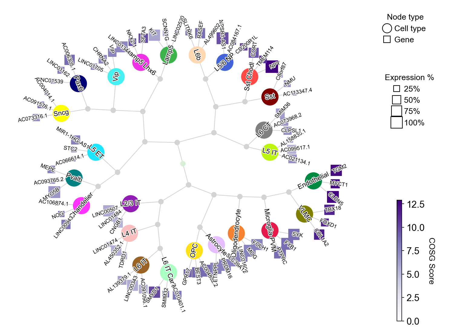
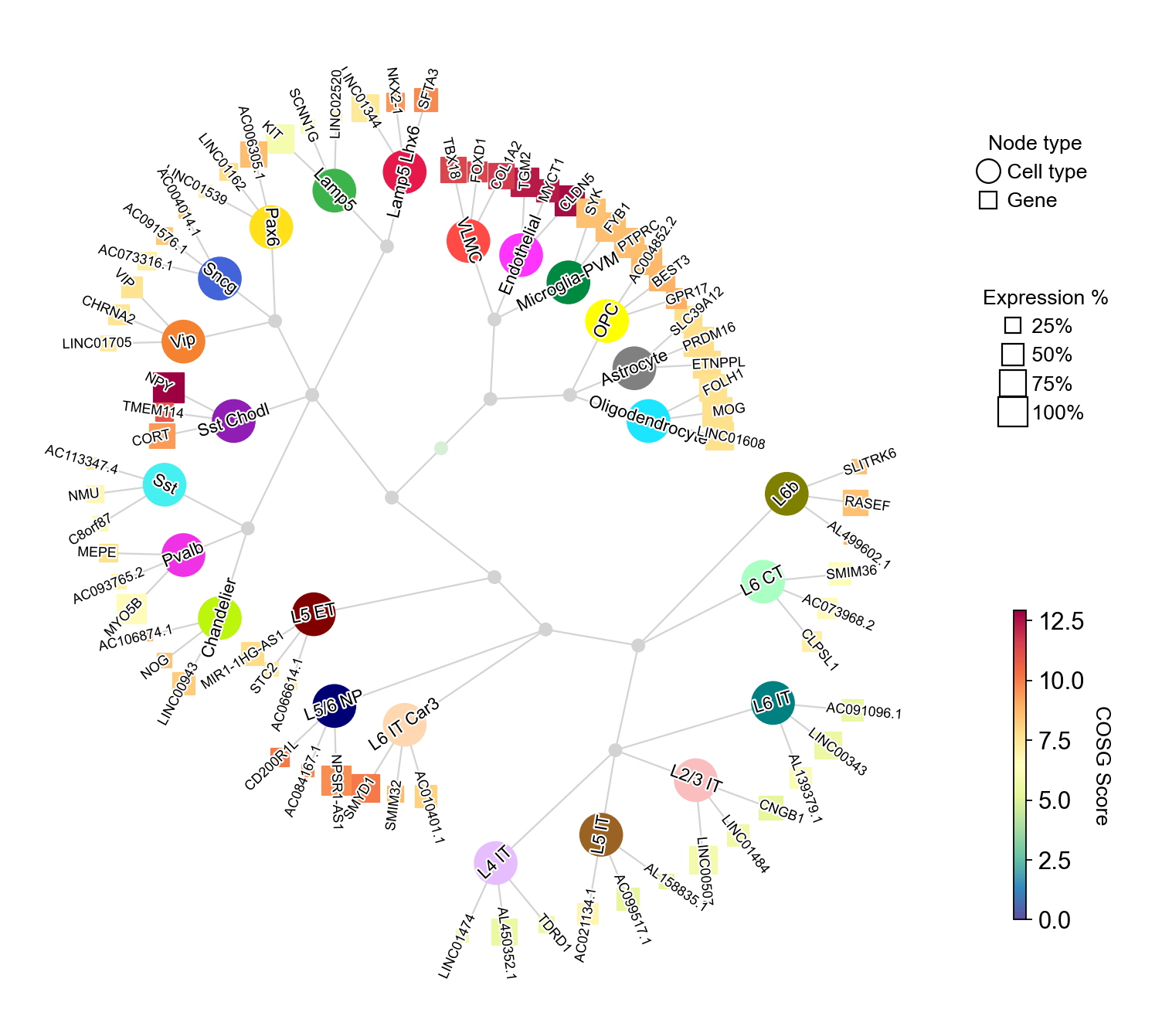
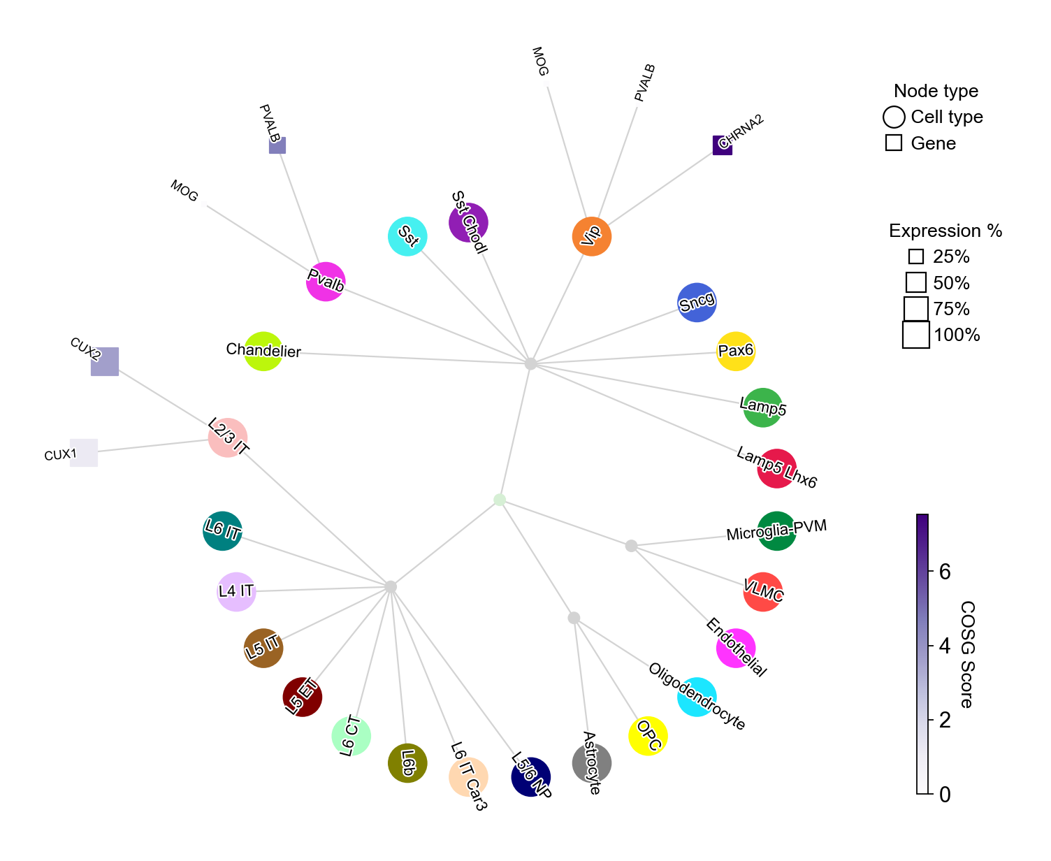
Visualizing the marker genes with plotMarkerDendrogram#

COSG provides an intutive visualization with marker gene names, COSG scores and cell cluster similarities:

[23]:

cosg.plotMarkerDendrogram(
     adata,
     group_by="Subclass",
     use_rep="X_scVI",
     calculate_dendrogram_on_cosg_scores=False,
     top_n_genes=3,
     radius_step=1.5,
     cmap="Purples",
     gene_label_offset=0.25,
     gene_label_color="black",
     linkage_method="ward",
     distance_metric="correlation",
     hierarchy_merge_scale=0,
     # collapse_scale=0.2,
     add_cluster_node_for_single_node_cluster=True,
     palette=None,
     figure_size= (10, 10),
     # node_shape_cell_type='o',
     # node_shape_gene='s',
     colorbar_width=0.01,
     gene_color_min=0,
     gene_color_max=None,
     show_figure=True,
     # save='./markerDendrogram.pdf',
)

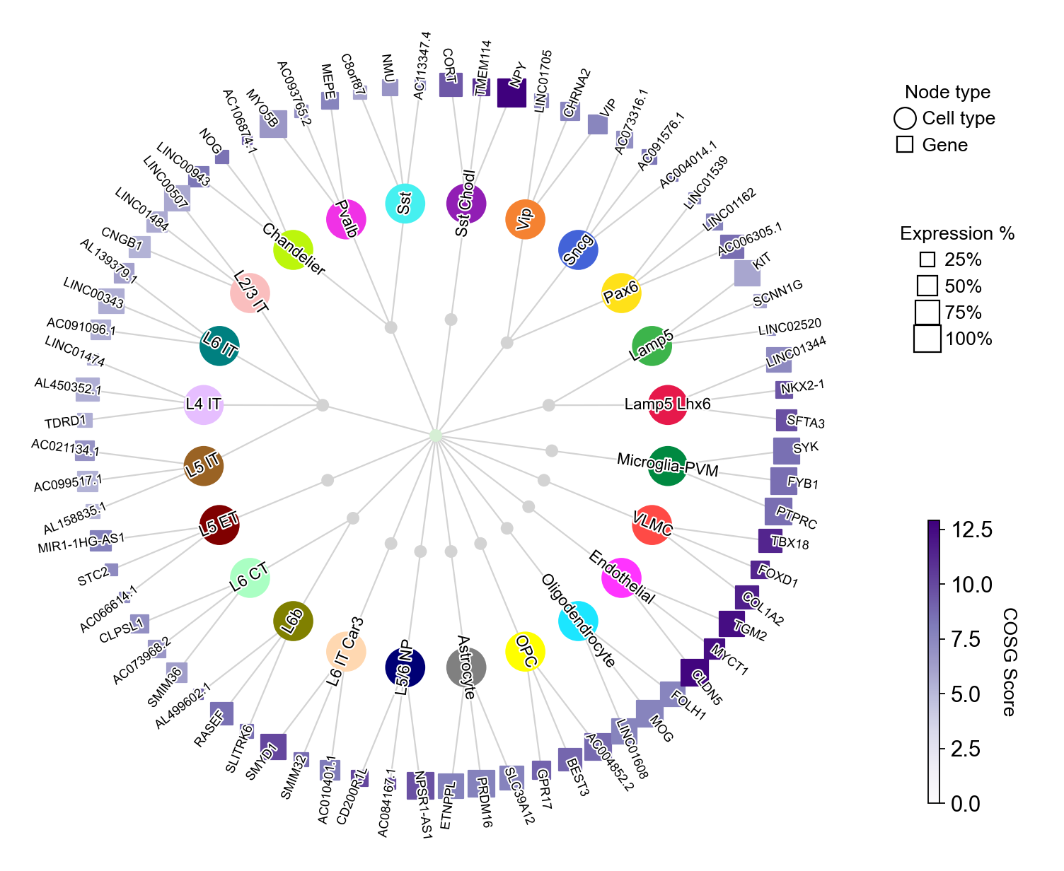
../_images/notebooks_24_COSG_tutorial_45_0.png

You could set the gene node colors by cmap and merge the hierarchical dendrogram by hierarchy_merge_scale. The parameter hierarchy_merge_scale (0 to 1) controls merging binary nodes into multi-child nodes based on distance similarity:

[24]:

cosg.plotMarkerDendrogram(
     adata,
     group_by="Subclass",
     use_rep="X_scVI",
     calculate_dendrogram_on_cosg_scores=True,
     top_n_genes=3,
     radius_step=1.5,
     cmap="Spectral_r",
     gene_label_offset=0.25,
     gene_label_color="black",
     linkage_method="ward",
     distance_metric="correlation",
     hierarchy_merge_scale=0.2,
     # collapse_scale=0.2,
     add_cluster_node_for_single_node_cluster=True,
     palette=None,
     figure_size= (10, 10),
     # figure_size= (8, 8),
     # node_shape_cell_type='o',
     # node_shape_gene='s',
     colorbar_width=0.01,
     gene_color_min=0,
     gene_color_max=None,
     show_figure=True,
     # save='./markerDendrogram.pdf',
)

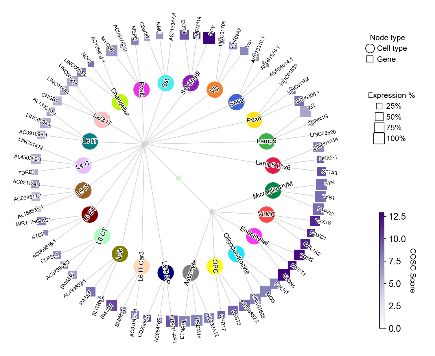
../_images/notebooks_24_COSG_tutorial_47_0.png

You could also collapse the dendrogram by setting collapse_scale to a value between 0 and 1:

[25]:

cosg.plotMarkerDendrogram(
     adata,
     group_by="Subclass",
     use_rep="X_scVI",
     calculate_dendrogram_on_cosg_scores=True,
     top_n_genes=3,
     radius_step=1.5,
     cmap="Purples",
     gene_label_offset=0.25,
     gene_label_color="black",
     linkage_method="ward",
     distance_metric="correlation",
     hierarchy_merge_scale=0,
     collapse_scale=0.2,
     add_cluster_node_for_single_node_cluster=True,
     palette=None,
     figure_size= (10, 10),
     # node_shape_cell_type='o',
     # node_shape_gene='s',
     colorbar_width=0.01,
     gene_color_min=0,
     gene_color_max=None,
     show_figure=True,
     # save='./markerDendrogram.pdf',
)

../_images/notebooks_24_COSG_tutorial_49_0.png

The parameter collapse_scale controls the clustering resolution of cell types, larger values lead to more clusters:

[26]:

cosg.plotMarkerDendrogram(
     adata,
     group_by="Subclass",
     use_rep="X_scVI",
     calculate_dendrogram_on_cosg_scores=True,
     top_n_genes=3,
     radius_step=1.5,
     cmap="Purples",
     gene_label_offset=0.25,
     gene_label_color="black",
     linkage_method="ward",
     distance_metric="correlation",
     hierarchy_merge_scale=0,
     collapse_scale=0.8,
     add_cluster_node_for_single_node_cluster=True,
     palette=None,
     figure_size= (10, 10),
     # node_shape_cell_type='o',
     # node_shape_gene='s',
     colorbar_width=0.01,
     gene_color_min=0,
     gene_color_max=None,
     show_figure=True,
     # save='./markerDendrogram.pdf',
)

../_images/notebooks_24_COSG_tutorial_51_0.png

Besides, you could also not show the figure by setting show_figure=False and save the figure as a PDF file by save='./markerDendrogram.pdf':

[27]:

cosg.plotMarkerDendrogram(
     adata,
     group_by="Subclass",
     use_rep="X_scVI",
     calculate_dendrogram_on_cosg_scores=True,
     top_n_genes=3,
     radius_step=1.5,
     cmap="Purples",
     gene_label_offset=0.25,
     gene_label_color="black",
     linkage_method="ward",
     distance_metric="correlation",
     hierarchy_merge_scale=0,
     collapse_scale=0.2,
     add_cluster_node_for_single_node_cluster=True,
     palette=None,
     figure_size= (10, 10),
     # node_shape_cell_type='o',
     # node_shape_gene='s',
     colorbar_width=0.01,
     gene_color_min=0,
     gene_color_max=None,
     show_figure=False,
     # save='./markerDendrogram.pdf',
)

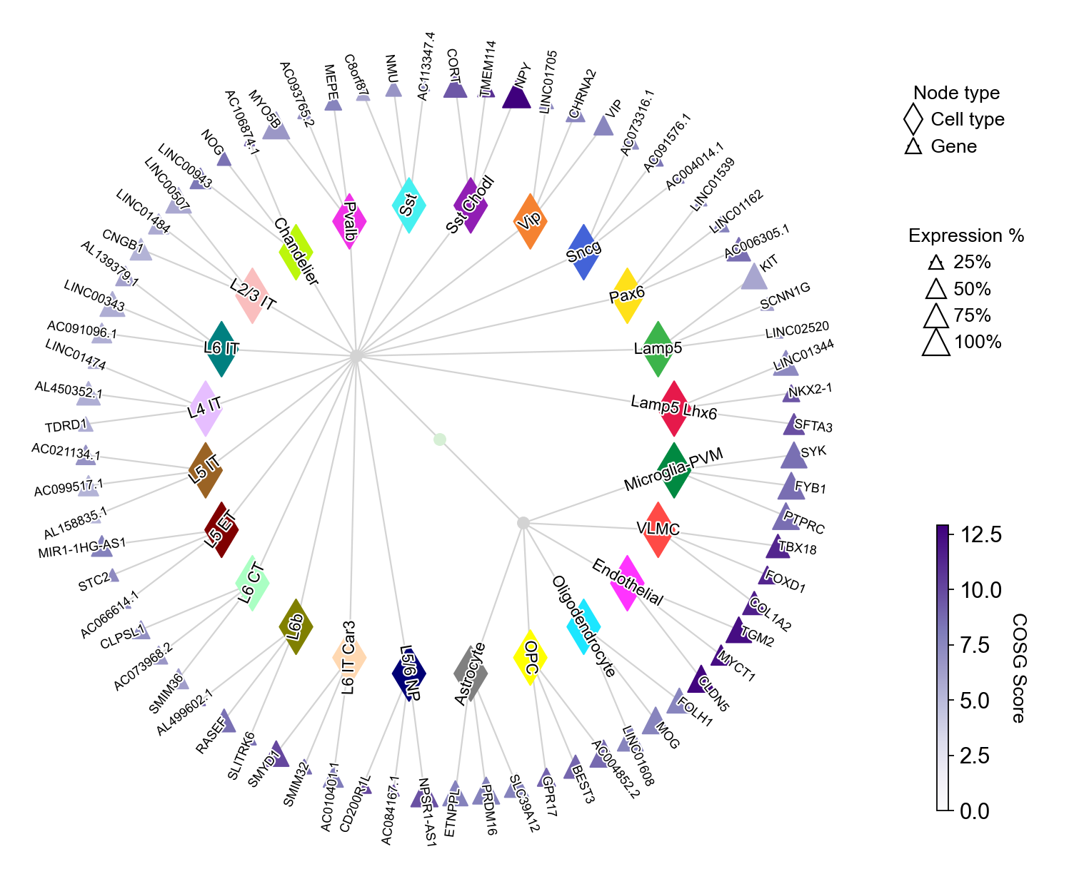
The shape of cell type nodes and gene nodes could be adjusted via node_shape_cell_type and node_shape_gene, respectively:

[28]:

cosg.plotMarkerDendrogram(
     adata,
     group_by="Subclass",
     use_rep="X_scVI",
     calculate_dendrogram_on_cosg_scores=True,
     top_n_genes=3,
     radius_step=1.5,
     cmap="Purples",
     gene_label_offset=0.25,
     gene_label_color="black",
     linkage_method="ward",
     distance_metric="correlation",
     hierarchy_merge_scale=0,
     collapse_scale=0.8,
     add_cluster_node_for_single_node_cluster=True,
     palette=None,
     figure_size= (10, 10),
     node_shape_cell_type='d',
     node_shape_gene='^',
     colorbar_width=0.01,
     gene_color_min=0,
     gene_color_max=None,
     show_figure=True,
     # save='./markerDendrogram.pdf',
)

../_images/notebooks_24_COSG_tutorial_55_0.png

Use customized cell type-gene pairs for visualization#

[29]:

celltype_gene_mapping={
    'L2/3 IT': ['CUX2', 'CUX1'],
    'Pvalb': ['PVALB', 'MOG', ],
    'Vip': ['CHRNA2', 'PVALB', 'MOG', ],
}

[30]:

cosg.plotMarkerDendrogram(
     adata,
     group_by="Subclass",
     use_rep="X_scVI",
     calculate_dendrogram_on_cosg_scores=True,
     top_n_genes=3,
     map_cell_type_gene=celltype_gene_mapping,
     cell_type_selected=None,
     radius_step=1.5,
     # cmap="Spectral_r",
     # cmap="magma_r",
     cmap="Purples",
     gene_label_offset=0.25,
     gene_label_color="black",
     linkage_method="ward",
     distance_metric="correlation",
     # hierarchy_merge_scale=0.2,
     collapse_scale=0.5,
     add_cluster_node_for_single_node_cluster=False,
     palette=None,
     figure_size= (10, 10),
     # node_shape_cell_type='o',
     # node_shape_gene='s',
     colorbar_width=0.01,
     gene_color_min=0,
     gene_color_max=None,
     # edge_curved=0.5,
     show_figure=True,

     # save='./markerDendrogram.pdf',
)

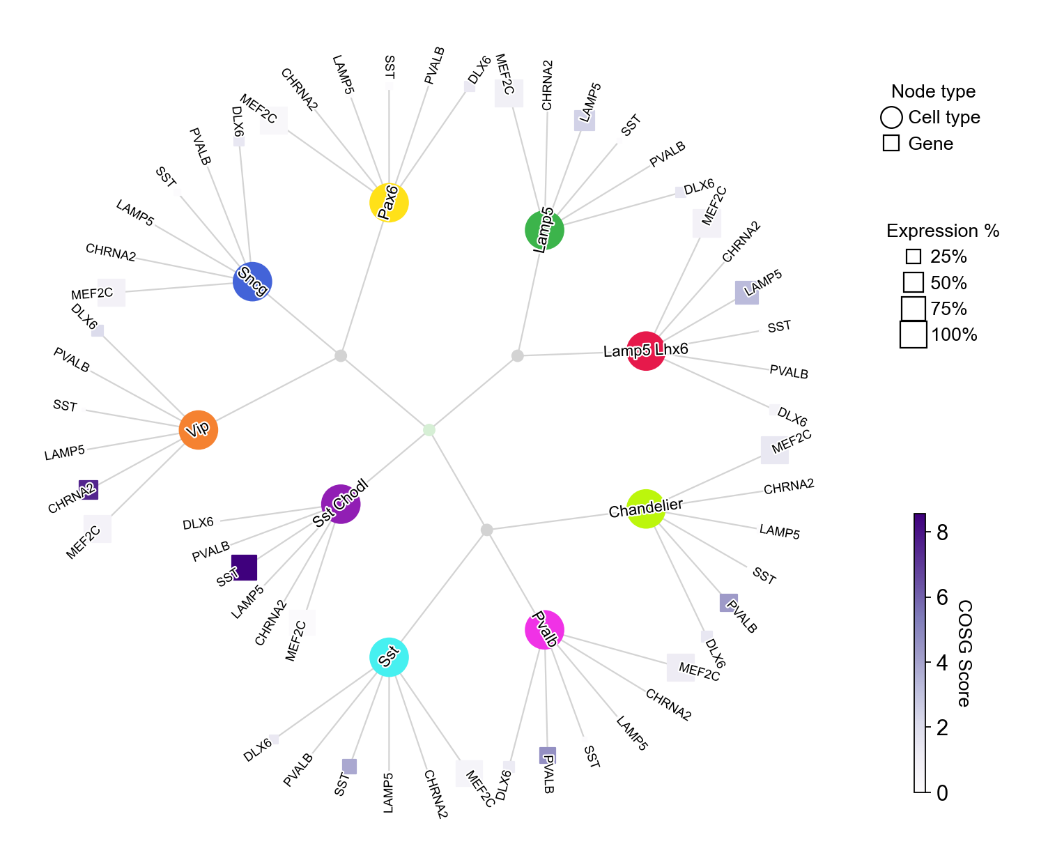
../_images/notebooks_24_COSG_tutorial_58_0.png

We could also combine the cell type filtering via cell_type_selected with customized cell type-gene pairs:

[31]:

celltype_gene_mapping={cell_type: ['DLX6', 'PVALB', 'SST',  'LAMP5',  'CHRNA2', 'MEF2C' ] for cell_type in adata.obs['Subclass'].cat.categories}

[32]:

cosg.plotMarkerDendrogram(
     adata,
     group_by="Subclass",
     use_rep="X_scVI",
     calculate_dendrogram_on_cosg_scores=True,
     top_n_genes=3,
     map_cell_type_gene=celltype_gene_mapping,
     cell_type_selected=['Lamp5 Lhx6', 'Lamp5', 'Pax6', 'Sncg', 'Vip', 'Sst Chodl', 'Sst',
       'Pvalb', 'Chandelier',],
     radius_step=1.5,
     # cmap="Spectral_r",
     # cmap="magma_r",
     cmap="Purples",
     gene_label_offset=0.25,
     gene_label_color="black",
     linkage_method="ward",
     distance_metric="correlation",
     # hierarchy_merge_scale=0.2,
     collapse_scale=0.5,
     add_cluster_node_for_single_node_cluster=False,
     palette=None,
     figure_size= (10, 10),
     # node_shape_cell_type='o',
     # node_shape_gene='s',
     colorbar_width=0.01,
     gene_color_min=0,
     gene_color_max=None,
     # edge_curved=0.5,
     show_figure=True,

     # save='./markerDendrogram.pdf',
)

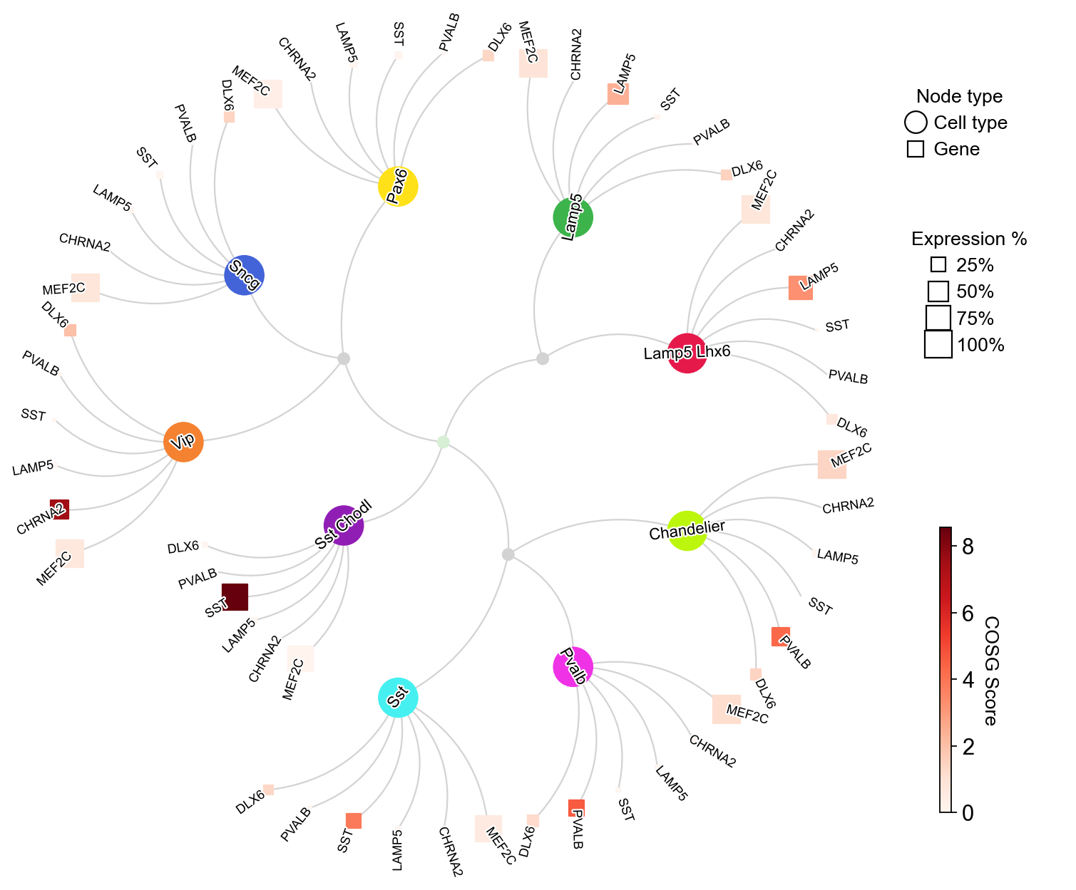
../_images/notebooks_24_COSG_tutorial_61_0.png

We can also change the curvature of edges via edge_curved:

[33]:

cosg.plotMarkerDendrogram(
     adata,
     group_by="Subclass",
     use_rep="X_scVI",
     calculate_dendrogram_on_cosg_scores=True,
     top_n_genes=3,
     map_cell_type_gene=celltype_gene_mapping,
     cell_type_selected=['Lamp5 Lhx6', 'Lamp5', 'Pax6', 'Sncg', 'Vip', 'Sst Chodl', 'Sst',
       'Pvalb', 'Chandelier',],
     radius_step=1.5,
     # cmap="Spectral_r",
     # cmap="magma_r",
     cmap="Reds",
     gene_label_offset=0.25,
     gene_label_color="black",
     linkage_method="ward",
     distance_metric="correlation",
     # hierarchy_merge_scale=0.2,
     collapse_scale=0.5,
     add_cluster_node_for_single_node_cluster=False,
     palette=None,
     figure_size= (10, 10),
     # node_shape_cell_type='o',
     # node_shape_gene='s',
     colorbar_width=0.01,
     gene_color_min=0,
     gene_color_max=None,
     edge_curved=0.5,
     show_figure=True,

     # save='./markerDendrogram.pdf',
)

../_images/notebooks_24_COSG_tutorial_63_0.png

Run COSG with assigned `batch_key`#

In this example dataset, the cells are divided into two groups based on whther the donors are severly affected, and the information is in the Severely Affected Donor column:

[34]:

pd.crosstab(adata.obs['Severely Affected Donor'], adata.obs['Subclass'])

[34]:

Subclass	Lamp5 Lhx6	Lamp5	Pax6	Sncg	Vip	Sst Chodl	Sst	Pvalb	Chandelier	L2/3 IT	...	L6 CT	L6b	L6 IT Car3	L5/6 NP	Astrocyte	OPC	Oligodendrocyte	Endothelial	VLMC	Microglia-PVM
Severely Affected Donor
N	285	598	134	312	1463	31	752	1246	146	4635	...	221	212	319	286	917	467	1578	26	77	563
Y	20	55	6	17	88	0	28	53	11	191	...	10	12	35	13	163	29	85	5	9	75

2 rows × 24 columns

[35]:

sc.pl.embedding(adata,
    basis='X_umap',
    color=['Severely Affected Donor'],
    palette=self_palette2,
    legend_fontoutline=2,
    legend_fontsize=7,
    legend_fontweight=5,
    # legend_loc='on data',
    # cmap='Spectral_r',
    ncols=3,
    size=10,
    frameon=False)

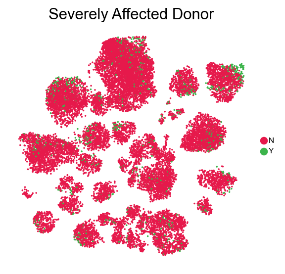
../_images/notebooks_24_COSG_tutorial_67_0.png

We could run COSG with batch_key set as “Severely Affected Donor”, computing cosine similarities separately for each batch before averaging them. The COSG scores were then derived from these averaged similarities.

[36]:

%%time
groupby='Subclass'
cosg.cosg(adata,
    key_added='cosg_batch',
    # use_raw=False, layer='log1p', ## e.g., if you want to use the log1p layer in adata
    mu=100,
    batch_key='Severely Affected Donor', ### Set the batch key
    batch_cell_number_threshold=5, ### Minimum number of cells required in a batch for a given cluster to be considered
    expressed_pct=0.1,
    remove_lowly_expressed=True,
    n_genes_user=adata.n_vars, ### Use all the genes, to enable the calculation of transformed COSG scores
    # n_genes_user=100,
    groupby=groupby,
    return_by_group=True,
    verbosity=1
)

Finished identifying marker genes by COSG, and the results are in adata.uns['cosg_batch'].
CPU times: user 8.06 s, sys: 3.47 s, total: 11.5 s
Wall time: 11.5 s

[37]:

pd.DataFrame(adata.uns['cosg_batch']['names']).head()

[37]:

	Lamp5 Lhx6	Lamp5	Pax6	Sncg	Vip	Sst Chodl	Sst	Pvalb	Chandelier	L2/3 IT	...	L6 CT	L6b	L6 IT Car3	L5/6 NP	Astrocyte	OPC	Oligodendrocyte	Endothelial	VLMC	Microglia-PVM
0	NKX2-1	LINC02520	AC006305.1	AC004014.1	LINC01705	NPY	NMU	MEPE	AC006065.4	LINC00507	...	CLPSL1	AL499602.1	SMYD1	AC084167.1	PRDM16	AC004852.2	LINC01608	CLDN5	COL1A2	PTPRC
1	SFTA3	SCNN1G	NTF3	AC091576.1	VIP	TMEM114	AC113347.4	MYO5B	AC106874.1	LINC01484	...	AC073968.2	AL357509.1	DCSTAMP	NPSR1-AS1	OBI1-AS1	GPR17	FOLH1	TGM2	TBX18	SYK
2	LINC01344	CPLX3	AL139090.1	AC073316.1	AJ006995.1	GHRH	LINC02133	AC093765.2	SCUBE3	AC008574.1	...	AC127459.2	RASEF	SMIM32	LINC02543	SLC39A12	BEST3	CD22	MYCT1	FMO2	FYB1
3	HCRTR2	AC099482.2	RELN	AL161629.1	LINC02257	SST	C8orf87	LRRC38	LINC00943	CNGB1	...	AC092114.1	LINC01654	AC010401.1	NPSR1	ETNPPL	FERMT1	MOG	CD34	FOXD1	IKZF1
4	MYB	KIT	LINC01539	LINC02408	NPR3	CORT	PAWR	SULF1	NOG	LINC02714	...	SEMA3E	AL596257.1	TRPC7-AS1	CD200R1L	SLC14A1	AC007106.1	SH3TC2	PCAT19	C7	DOCK8

5 rows × 24 columns

and here are the COSG results without batch_key assigned:

[38]:

pd.DataFrame(adata.uns['cosg']['names']).head()

[38]:

	Lamp5 Lhx6	Lamp5	Pax6	Sncg	Vip	Sst Chodl	Sst	Pvalb	Chandelier	L2/3 IT	...	L6 CT	L6b	L6 IT Car3	L5/6 NP	Astrocyte	OPC	Oligodendrocyte	Endothelial	VLMC	Microglia-PVM
0	SFTA3	LINC02520	AC006305.1	AC004014.1	VIP	NPY	AC113347.4	MEPE	AC106874.1	LINC00507	...	CLPSL1	AL499602.1	SMYD1	CD200R1L	ETNPPL	GPR17	LINC01608	CLDN5	COL1A2	PTPRC
1	NKX2-1	SCNN1G	LINC01162	AC091576.1	CHRNA2	TMEM114	NMU	AC093765.2	NOG	LINC01484	...	AC073968.2	RASEF	SMIM32	AC084167.1	PRDM16	BEST3	MOG	MYCT1	FOXD1	FYB1
2	LINC01344	KIT	LINC01539	AC073316.1	LINC01705	CORT	C8orf87	MYO5B	LINC00943	CNGB1	...	SMIM36	SLITRK6	AC010401.1	NPSR1-AS1	SLC39A12	AC004852.2	FOLH1	TGM2	TBX18	SYK
3	AL355482.1	AC099482.2	ABCB5	AL161629.1	AJ006995.1	GHRH	LINC02133	LRRC38	AC006065.4	AC008574.1	...	KL	SCUBE1	AC073225.1	LINC02042	OBI1-AS1	LINC01546	CD22	SRARP	C7	IKZF1
4	HCRTR2	CPLX3	LINC01416	AC004862.1	NPR3	DDC	OTOF	AC006364.1	SCUBE3	LINC02714	...	AC092114.1	FIBCD1	DCSTAMP	NPSR1	SLC14A1	VCAN-AS1	SLCO1A2	FENDRR	FMO2	PIK3R5

5 rows × 24 columns

Save the data#

[39]:

adata.write(save_dir+'/'+prefix+'.h5ad')

[40]:

adata

[40]:

AnnData object with n_obs × n_vars = 20000 × 36601
    obs: 'sample_id', 'Neurotypical reference', 'Donor ID', 'Organism', 'Brain Region', 'Sex', 'Gender', 'Age at Death', 'Race (choice=White)', 'Race (choice=Black/ African American)', 'Race (choice=Asian)', 'Race (choice=American Indian/ Alaska Native)', 'Race (choice=Native Hawaiian or Pacific Islander)', 'Race (choice=Unknown or unreported)', 'Race (choice=Other)', 'specify other race', 'Hispanic/Latino', 'Highest level of education', 'Years of education', 'PMI', 'Fresh Brain Weight', 'Brain pH', 'Overall AD neuropathological Change', 'Thal', 'Braak', 'CERAD score', 'Overall CAA Score', 'Highest Lewy Body Disease', 'Total Microinfarcts (not observed grossly)', 'Total microinfarcts in screening sections', 'Atherosclerosis', 'Arteriolosclerosis', 'LATE', 'Cognitive Status', 'Last CASI Score', 'Interval from last CASI in months', 'Last MMSE Score', 'Interval from last MMSE in months', 'Last MOCA Score', 'Interval from last MOCA in months', 'APOE Genotype', 'Primary Study Name', 'Secondary Study Name', 'NeuN positive fraction on FANS', 'RIN', 'cell_prep_type', 'facs_population_plan', 'rna_amplification', 'sample_name', 'sample_quantity_count', 'expc_cell_capture', 'method', 'pcr_cycles', 'percent_cdna_longer_than_400bp', 'rna_amplification_pass_fail', 'amplified_quantity_ng', 'load_name', 'library_prep', 'library_input_ng', 'r1_index', 'avg_size_bp', 'quantification_fmol', 'library_prep_pass_fail', 'exp_component_vendor_name', 'batch_vendor_name', 'experiment_component_failed', 'alignment', 'Genome', 'ar_id', 'bc', 'GEX_Estimated_number_of_cells', 'GEX_number_of_reads', 'GEX_sequencing_saturation', 'GEX_Mean_raw_reads_per_cell', 'GEX_Q30_bases_in_barcode', 'GEX_Q30_bases_in_read_2', 'GEX_Q30_bases_in_UMI', 'GEX_Percent_duplicates', 'GEX_Q30_bases_in_sample_index_i1', 'GEX_Q30_bases_in_sample_index_i2', 'GEX_Reads_with_TSO', 'GEX_Sequenced_read_pairs', 'GEX_Valid_UMIs', 'GEX_Valid_barcodes', 'GEX_Reads_mapped_to_genome', 'GEX_Reads_mapped_confidently_to_genome', 'GEX_Reads_mapped_confidently_to_intergenic_regions', 'GEX_Reads_mapped_confidently_to_intronic_regions', 'GEX_Reads_mapped_confidently_to_exonic_regions', 'GEX_Reads_mapped_confidently_to_transcriptome', 'GEX_Reads_mapped_antisense_to_gene', 'GEX_Fraction_of_transcriptomic_reads_in_cells', 'GEX_Total_genes_detected', 'GEX_Median_UMI_counts_per_cell', 'GEX_Median_genes_per_cell', 'Multiome_Feature_linkages_detected', 'Multiome_Linked_genes', 'Multiome_Linked_peaks', 'ATAC_Confidently_mapped_read_pairs', 'ATAC_Fraction_of_genome_in_peaks', 'ATAC_Fraction_of_high_quality_fragments_in_cells', 'ATAC_Fraction_of_high_quality_fragments_overlapping_TSS', 'ATAC_Fraction_of_high_quality_fragments_overlapping_peaks', 'ATAC_Fraction_of_transposition_events_in_peaks_in_cells', 'ATAC_Mean_raw_read_pairs_per_cell', 'ATAC_Median_high_quality_fragments_per_cell', 'ATAC_Non-nuclear_read_pairs', 'ATAC_Number_of_peaks', 'ATAC_Percent_duplicates', 'ATAC_Q30_bases_in_barcode', 'ATAC_Q30_bases_in_read_1', 'ATAC_Q30_bases_in_read_2', 'ATAC_Q30_bases_in_sample_index_i1', 'ATAC_Sequenced_read_pairs', 'ATAC_TSS_enrichment_score', 'ATAC_Unmapped_read_pairs', 'ATAC_Valid_barcodes', 'Number of mapped reads', 'Number of unmapped reads', 'Number of multimapped reads', 'Number of reads', 'Number of UMIs', 'Genes detected', 'Doublet score', 'Fraction mitochondrial UMIs', 'Used in analysis', 'Class confidence', 'Class', 'Subclass confidence', 'Subclass', 'Supertype confidence', 'Supertype (non-expanded)', 'Supertype', 'Continuous Pseudo-progression Score', 'Severely Affected Donor'
    var: 'gene_ids'
    uns: 'APOE4 Status_colors', 'Braak_colors', 'CERAD score_colors', 'Cognitive Status_colors', 'Great Apes Metadata', 'Highest Lewy Body Disease_colors', 'LATE_colors', 'Overall AD neuropathological Change_colors', 'Sex_colors', 'Subclass_colors', 'Supertype_colors', 'Thal_colors', 'UW Clinical Metadata', 'X_normalization', 'batch_condition', 'default_embedding', 'neighbors', 'title', 'umap', 'cosg', 'dendrogram_Subclass', 'Severely Affected Donor_colors', 'cosg_batch'
    obsm: 'X_scVI', 'X_umap'
    layers: 'UMIs'
    obsp: 'connectivities', 'distances'

[ ]:

Table of Contents

Marker gene identification with COSG#

Setting basics#

Setting colors#

Setting paths#

Load the data#

Import COSG#

Calculate normalized COSG scores for each gene across all cell types#

Visualizing the marker genes with plotMarkerDendrogram#

Use customized cell type-gene pairs for visualization#

Run COSG with assigned batch_key#

Save the data#

Run COSG with assigned `batch_key`#