Introduction#
PIASO stands for Precise Intregrative Analysis of Single-cell Omics
Before starting the tutorial, ensure that PIASO is installed on your machine. If you haven’t installed it yet, follow the steps at Installing PIASO before proceeding.
[1]:
import numpy as np
import pandas as pd
import scanpy as sc
import os
import logging
from matplotlib import rcParams
from sklearn.model_selection import StratifiedShuffleSplit
from sklearn import metrics
from sklearn.metrics import f1_score
import seaborn as sns
import matplotlib.pyplot as plt
[2]:
path = '/home/vas744/Analysis/Python/Packages/PIASO'
import sys
sys.path.append(path)
path = '/home/vas744/Analysis/Python/Packages/COSG'
import sys
sys.path.append(path)
import piaso
import cosg
/home/vas744/.local/lib/python3.9/site-packages/networkx/utils/backends.py:135: RuntimeWarning: networkx backend defined more than once: nx-loopback
  backends.update(_get_backends("networkx.backends"))
[3]:
sc.set_figure_params(dpi=96,dpi_save=300, color_map='viridis',facecolor='white')
rcParams['font.sans-serif'] = "Arial"
rcParams['font.family'] = "Arial"
sc.settings.verbosity = 3
sc.logging.print_header()
scanpy==1.10.3 anndata==0.10.8 umap==0.5.7 numpy==1.26.4 scipy==1.13.0 pandas==2.2.3 scikit-learn==1.5.2 statsmodels==0.14.4 igraph==0.11.5 louvain==0.8.2 pynndescent==0.5.13
Load the data#
Let us load a 20k subsampled version of the Seattle Alzheimer’s Disease Brain Cell Atlas (SEA-AD) project dataset described in detail in Gabitto et. al. (2024). We will be using the scRNA-seq data from the dataset in this tutorial.
Download the subsampled dataset from Google Drive: https://drive.google.com/file/d/1EdRA0ECvPlEnNaOzKqj19GrEtucB7hmE/view?usp=drive_link
The original data is available on https://portal.brain-map.org/explore/seattle-alzheimers-disease.
[4]:
!/home/vas744/Software/gdrive files download --overwrite --destination /n/scratch/users/v/vas744/Data/Public/PIASO 1EdRA0ECvPlEnNaOzKqj19GrEtucB7hmE
Downloading SEA-AD_RNA_MTG_subsample_excludeReference_20k_piaso.h5ad
Successfully downloaded SEA-AD_RNA_MTG_subsample_excludeReference_20k_piaso.h5ad
[5]:
adata=sc.read('/n/scratch/users/v/vas744/Data/Public/PIASO/SEA-AD_RNA_MTG_subsample_excludeReference_20k_piaso.h5ad')
adata
[5]:
AnnData object with n_obs × n_vars = 20000 × 36601
    obs: 'sample_id', 'Neurotypical reference', 'Donor ID', 'Organism', 'Brain Region', 'Sex', 'Gender', 'Age at Death', 'Race (choice=White)', 'Race (choice=Black/ African American)', 'Race (choice=Asian)', 'Race (choice=American Indian/ Alaska Native)', 'Race (choice=Native Hawaiian or Pacific Islander)', 'Race (choice=Unknown or unreported)', 'Race (choice=Other)', 'specify other race', 'Hispanic/Latino', 'Highest level of education', 'Years of education', 'PMI', 'Fresh Brain Weight', 'Brain pH', 'Overall AD neuropathological Change', 'Thal', 'Braak', 'CERAD score', 'Overall CAA Score', 'Highest Lewy Body Disease', 'Total Microinfarcts (not observed grossly)', 'Total microinfarcts in screening sections', 'Atherosclerosis', 'Arteriolosclerosis', 'LATE', 'Cognitive Status', 'Last CASI Score', 'Interval from last CASI in months', 'Last MMSE Score', 'Interval from last MMSE in months', 'Last MOCA Score', 'Interval from last MOCA in months', 'APOE Genotype', 'Primary Study Name', 'Secondary Study Name', 'NeuN positive fraction on FANS', 'RIN', 'cell_prep_type', 'facs_population_plan', 'rna_amplification', 'sample_name', 'sample_quantity_count', 'expc_cell_capture', 'method', 'pcr_cycles', 'percent_cdna_longer_than_400bp', 'rna_amplification_pass_fail', 'amplified_quantity_ng', 'load_name', 'library_prep', 'library_input_ng', 'r1_index', 'avg_size_bp', 'quantification_fmol', 'library_prep_pass_fail', 'exp_component_vendor_name', 'batch_vendor_name', 'experiment_component_failed', 'alignment', 'Genome', 'ar_id', 'bc', 'GEX_Estimated_number_of_cells', 'GEX_number_of_reads', 'GEX_sequencing_saturation', 'GEX_Mean_raw_reads_per_cell', 'GEX_Q30_bases_in_barcode', 'GEX_Q30_bases_in_read_2', 'GEX_Q30_bases_in_UMI', 'GEX_Percent_duplicates', 'GEX_Q30_bases_in_sample_index_i1', 'GEX_Q30_bases_in_sample_index_i2', 'GEX_Reads_with_TSO', 'GEX_Sequenced_read_pairs', 'GEX_Valid_UMIs', 'GEX_Valid_barcodes', 'GEX_Reads_mapped_to_genome', 'GEX_Reads_mapped_confidently_to_genome', 'GEX_Reads_mapped_confidently_to_intergenic_regions', 'GEX_Reads_mapped_confidently_to_intronic_regions', 'GEX_Reads_mapped_confidently_to_exonic_regions', 'GEX_Reads_mapped_confidently_to_transcriptome', 'GEX_Reads_mapped_antisense_to_gene', 'GEX_Fraction_of_transcriptomic_reads_in_cells', 'GEX_Total_genes_detected', 'GEX_Median_UMI_counts_per_cell', 'GEX_Median_genes_per_cell', 'Multiome_Feature_linkages_detected', 'Multiome_Linked_genes', 'Multiome_Linked_peaks', 'ATAC_Confidently_mapped_read_pairs', 'ATAC_Fraction_of_genome_in_peaks', 'ATAC_Fraction_of_high_quality_fragments_in_cells', 'ATAC_Fraction_of_high_quality_fragments_overlapping_TSS', 'ATAC_Fraction_of_high_quality_fragments_overlapping_peaks', 'ATAC_Fraction_of_transposition_events_in_peaks_in_cells', 'ATAC_Mean_raw_read_pairs_per_cell', 'ATAC_Median_high_quality_fragments_per_cell', 'ATAC_Non-nuclear_read_pairs', 'ATAC_Number_of_peaks', 'ATAC_Percent_duplicates', 'ATAC_Q30_bases_in_barcode', 'ATAC_Q30_bases_in_read_1', 'ATAC_Q30_bases_in_read_2', 'ATAC_Q30_bases_in_sample_index_i1', 'ATAC_Sequenced_read_pairs', 'ATAC_TSS_enrichment_score', 'ATAC_Unmapped_read_pairs', 'ATAC_Valid_barcodes', 'Number of mapped reads', 'Number of unmapped reads', 'Number of multimapped reads', 'Number of reads', 'Number of UMIs', 'Genes detected', 'Doublet score', 'Fraction mitochondrial UMIs', 'Used in analysis', 'Class confidence', 'Class', 'Subclass confidence', 'Subclass', 'Supertype confidence', 'Supertype (non-expanded)', 'Supertype', 'Continuous Pseudo-progression Score', 'Severely Affected Donor'
    var: 'gene_ids'
    uns: 'APOE4 Status_colors', 'Braak_colors', 'CERAD score_colors', 'Cognitive Status_colors', 'Great Apes Metadata', 'Highest Lewy Body Disease_colors', 'LATE_colors', 'Overall AD neuropathological Change_colors', 'Sex_colors', 'Subclass_colors', 'Supertype_colors', 'Thal_colors', 'UW Clinical Metadata', 'X_normalization', 'batch_condition', 'default_embedding', 'neighbors', 'title', 'umap'
    obsm: 'X_scVI', 'X_umap'
    layers: 'UMIs'
    obsp: 'connectivities', 'distances'
This data has been pre-processed already. But for the purposes of this tutorial, we will start again with the counts data and go through the normalization and other pre-processing steps.
[6]:
adata.X=adata.layers['UMIs'].copy()
Now we filter out cells with less than 200 genes. You can also filter out genes that are lowly expressed in cells.
[7]:
sc.pp.filter_cells(adata, min_genes=200)
Identify and annotate the mitochondrial genes in the data and compute their quality control metrics.
[8]:
adata.var['mt'] = adata.var_names.str.startswith('MT-')  # annotate the group of mitochondrial genes as 'mt'
sc.pp.calculate_qc_metrics(adata, qc_vars=['mt'], percent_top=None, log1p=False, inplace=True)
Identify and annotate the ribosomal protein genes in the data and compute the percenatge of total genes that are ribosomal protein genes.
[9]:
ribo_cells = adata.var_names.str.startswith('RPS','RPL')
adata.obs['pct_counts_ribo'] = np.ravel(100*np.sum(adata[:, ribo_cells].X, axis = 1) / np.sum(adata.X, axis = 1))
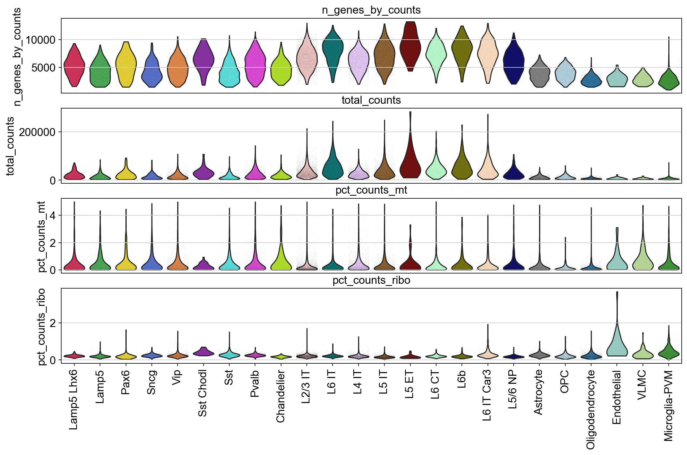
Visualize the metrics for all genes, and mitochondrial and ribosomal protein genes in a violin plot.
The levels of these genes can be used to eliminate low-quality cells. Higher percentage if mt or ribo genes in a cell implies a lysed cell prior to mRNA capture.
[10]:
piaso.pl.plot_features_violin(adata,
                              ['n_genes_by_counts', 'total_counts', 'pct_counts_mt','pct_counts_ribo'],
                              groupby='Subclass')
Normalize and log-transform the data#
Normalize each cell with the total counts over all the genes, and then logarithmize the data.
[11]:
adata.layers['raw']=adata.X.copy()

sc.pp.normalize_total(adata, target_sum=1e4)
sc.pp.log1p(adata)

adata.layers['log1p']=adata.X
normalizing counts per cell
    finished (0:00:00)
Now, we perform feature selection to reduce the number of fearures (genes) used as input for further downstream processing. Here, we select the top 3000 highly variable genes.
RNA-seq data is usually overdispersed, i.e. variance exceeds the mean. Therefore, we normalize such data by adjusting for overdispersion using Pearson residuals derived from the fitted negative binomial model.
Note: Since we aren’t filtering any genes here, there might be some genes which don’t express in any cell and therefore lead to columns with all zeros. This is the reason for the RuntimeWarning: invalid value encountered in divide residuals = diff / np.sqrt(mu + mu**2 / theta). But this will not affect our analysis, since we will be using the log1p layer instead of the raw layer.
[12]:
sc.experimental.pp.highly_variable_genes(adata,
                                         layer='raw',
                                         n_top_genes=3000)

pr_offset=sc.experimental.pp.normalize_pearson_residuals(adata,
                                                         layer='raw',
                                                         inplace=False)

adata.X=pr_offset['X']

del pr_offset
extracting highly variable genes
--> added
    'highly_variable', boolean vector (adata.var)
    'highly_variable_rank', float vector (adata.var)
    'highly_variable_nbatches', int vector (adata.var)
    'highly_variable_intersection', boolean vector (adata.var)
    'means', float vector (adata.var)
    'variances', float vector (adata.var)
    'residual_variances', float vector (adata.var)
computing analytic Pearson residuals on raw
/home/vas744/.local/lib/python3.9/site-packages/scanpy/experimental/pp/_normalization.py:70: RuntimeWarning: invalid value encountered in divide
  residuals = diff / np.sqrt(mu + mu**2 / theta)
finished (0:00:33)
Dimensionality reduction and visualization#
Again, since the data has been pre-processed, we have the umap computation given by the authors in the AnnData object, but for the purposes of this tutorial, we will backup that umap, and re-compute again.
[13]:
adata.obsm['X_umap_backup']=adata.obsm['X_umap'].copy()
[14]:
piaso.tl.runSVD(adata,
                   use_highly_variable=True,
                   n_components=50,
                   random_state=10,
                   key_added='X_svd')
[15]:
%%time
sc.pp.neighbors(adata,
                use_rep='X_svd',
                n_neighbors=15,
                random_state=10,
                knn=True,
                method="umap")
sc.tl.umap(adata)
computing neighbors
    finished: added to `.uns['neighbors']`
    `.obsp['distances']`, distances for each pair of neighbors
    `.obsp['connectivities']`, weighted adjacency matrix (0:00:38)
computing UMAP
    finished: added
    'X_umap', UMAP coordinates (adata.obsm)
    'umap', UMAP parameters (adata.uns) (0:00:36)
CPU times: user 5min 26s, sys: 843 ms, total: 5min 27s
Wall time: 1min 14s
[16]:
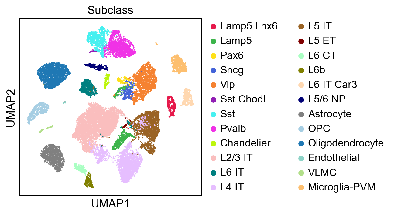
sc.pl.umap(adata,
           color=['Subclass'],
           palette=piaso.pl.color.d_color4,
           cmap=piaso.pl.color.c_color4,
           size=10,
           frameon=True)
Backup the umap computation based on the raw data.
[17]:
adata.obsm['X_umap_raw']=adata.obsm['X_umap'].copy()
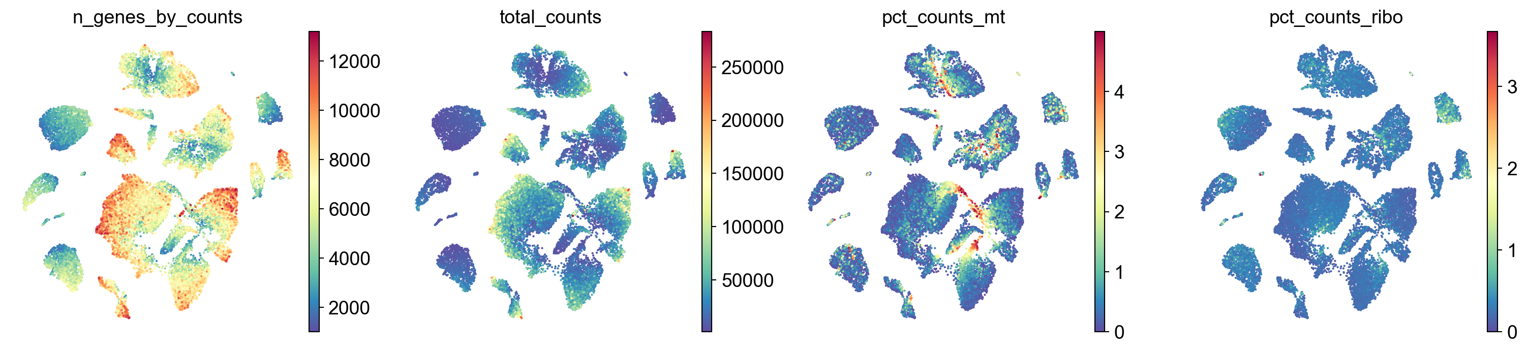
Visualize the overall as well as mitochondrial and ribosomal protein gene expression.
[18]:
sc.pl.umap(adata,
           color=['n_genes_by_counts', 'total_counts','pct_counts_mt','pct_counts_ribo'],
           cmap='Spectral_r',
           palette=piaso.pl.color.d_color4,
           ncols=4,
           size=10,
           frameon=False,)
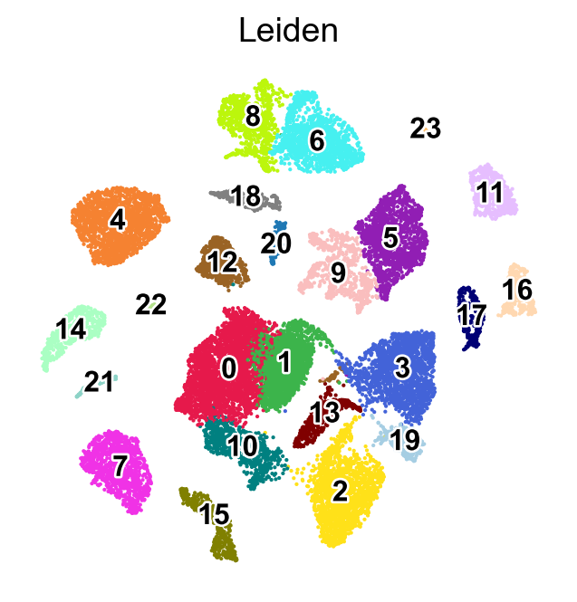
Cluster the data#
[19]:
%%time
sc.tl.leiden(adata,resolution=0.5,key_added='Leiden',flavor="leidenalg",n_iterations=-1)
running Leiden clustering
<timed eval>:1: FutureWarning: In the future, the default backend for leiden will be igraph instead of leidenalg.

 To achieve the future defaults please pass: flavor="igraph" and n_iterations=2.  directed must also be False to work with igraph's implementation.
    finished: found 24 clusters and added
    'Leiden', the cluster labels (adata.obs, categorical) (0:00:01)
CPU times: user 1.57 s, sys: 40.1 ms, total: 1.61 s
Wall time: 1.61 s
[20]:
logging.getLogger('matplotlib.font_manager').disabled = True
[21]:
sc.pl.umap(adata,
           color=['Leiden'],
           palette=piaso.pl.color.d_color4,
           cmap=piaso.pl.color.c_color4,
           legend_fontsize=12,
           legend_fontoutline=2,
           legend_loc='on data',
           size=10,
           frameon=False)

Identify marker genes for every cluster#
In this workflow, you might want to identify marker genes for each cluster. This can be done using cosg Dai et. al. (2022), which is a python package you can install in your environment by running:
pip install cosg
For more details about cosg, please refer to:
[22]:
n_gene=30
cosg.cosg(adata,
          key_added='cosg',
          use_raw=False,
          layer='log1p',
          mu=100,
          expressed_pct=0.1,
          remove_lowly_expressed=True,
          n_genes_user=100,
          groupby='Leiden')
[23]:
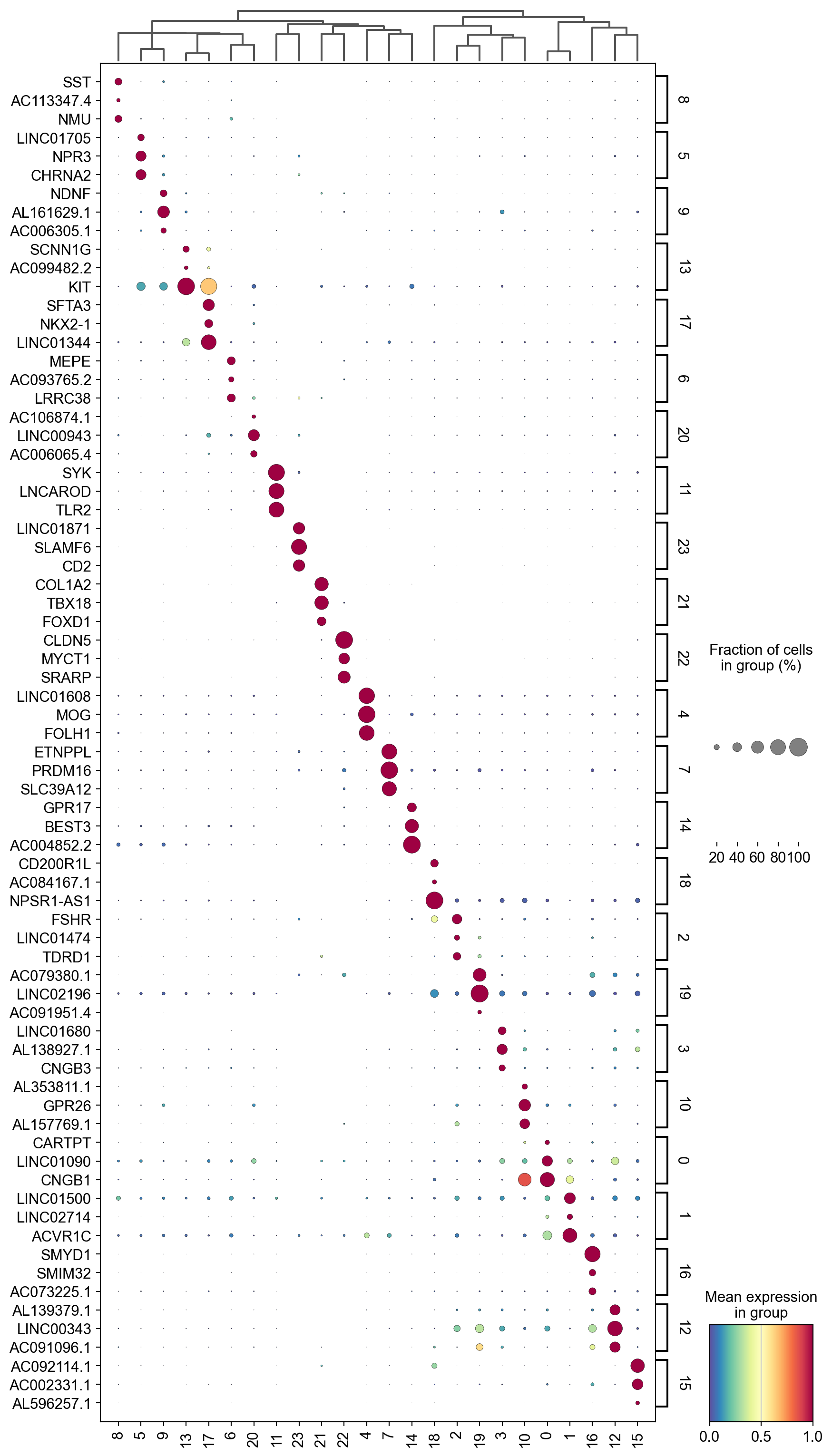
sc.tl.dendrogram(adata,groupby='Leiden',use_rep='X_svd')
df_tmp=pd.DataFrame(adata.uns['cosg']['names'][:3,]).T
df_tmp=df_tmp.reindex(adata.uns['dendrogram_'+'Leiden']['categories_ordered'])
marker_genes_list={idx: list(row.values) for idx, row in df_tmp.iterrows()}
marker_genes_list = {k: v for k, v in marker_genes_list.items() if not any(isinstance(x, float) for x in v)}

sc.pl.dotplot(adata,
              marker_genes_list,
              groupby='Leiden',
              layer='log1p',
              dendrogram=True,
              swap_axes=True,
              standard_scale='var',
              cmap='Spectral_r',
              figsize=[10,20])
Storing dendrogram info using `.uns['dendrogram_Leiden']`
[24]:
marker_gene=pd.DataFrame(adata.uns['cosg']['names'])

sc.pl.umap(adata,
           color=['Leiden'],
           palette=piaso.pl.color.d_color4,
           cmap=piaso.pl.color.c_color4,
           legend_fontsize=12,
           legend_fontoutline=2,
           legend_loc='on data',
           size=10,
           frameon=False)
Run GDR for dimensionality reduction#
GDR (marker Gene-guided Dimensionality Reduction) is an alternative dimensionality reduction method by projecting cells into a low-dimensional gene expression space that reflects biological identity in each dimension. Here we will demonstrate how PIASO’s runGDR can be used instead of SVD for dimensionality reduction.
For more details about GDR and it’s applications, please refer to: https://www.biorxiv.org/content/10.1101/2024.07.20.604399v1
[25]:
adata.obsm['X_umap_svd']=adata.obsm['X_umap'].copy()
[26]:
piaso.tl.runGDR(adata,
                batch_key=None,
                groupby='Leiden',
                n_gene=30,
                mu=1.0,
                use_highly_variable=True,
                n_highly_variable_genes=5000,
                layer='log1p',
                score_layer='log1p',
                n_svd_dims=50,
                resolution=1.0,
                scoring_method=None,
                key_added='X_gdr',
                verbosity=0)
GDR embeddings saved to adata.obsm['X_gdr']
[27]:
%%time
sc.pp.neighbors(adata,
                use_rep='X_gdr',
                n_neighbors=15,
                random_state=10,
                knn=True,
                method="umap")
sc.tl.umap(adata)
computing neighbors
    finished: added to `.uns['neighbors']`
    `.obsp['distances']`, distances for each pair of neighbors
    `.obsp['connectivities']`, weighted adjacency matrix (0:00:04)
computing UMAP
    finished: added
    'X_umap', UMAP coordinates (adata.obsm)
    'umap', UMAP parameters (adata.uns) (0:00:30)
CPU times: user 2min 46s, sys: 565 ms, total: 2min 47s
Wall time: 34.7 s
[28]:
sc.pl.umap(adata,
           color=['Subclass'],
           palette=piaso.pl.color.d_color4,
           cmap=piaso.pl.color.c_color4,
           ncols=1,
           size=10,
           frameon=True)
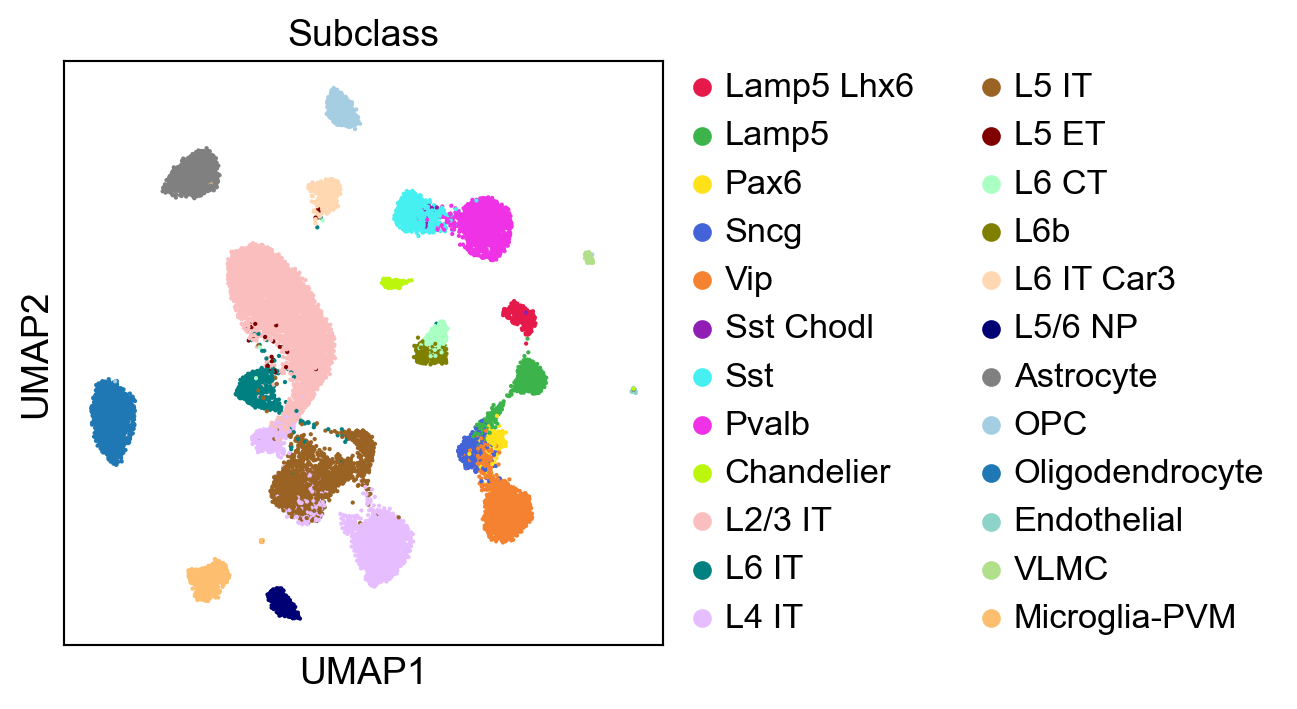
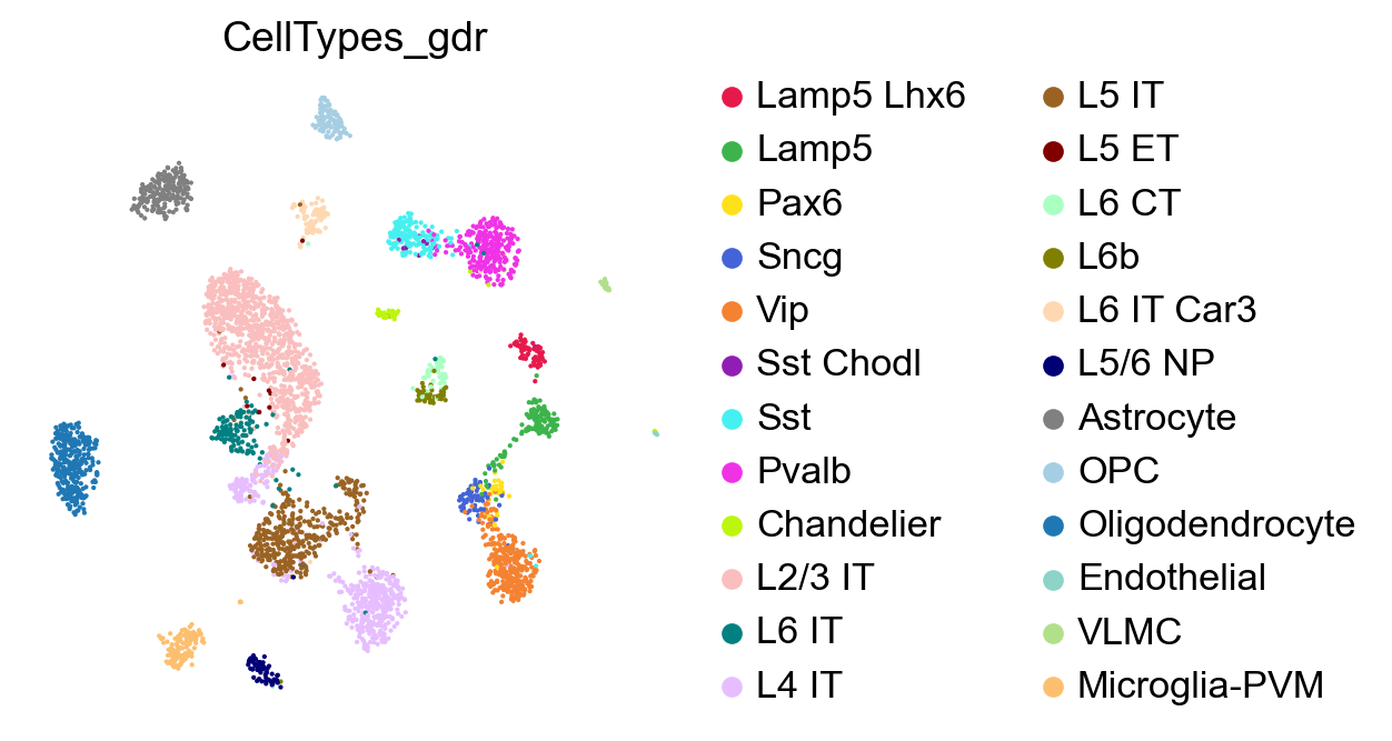
Predict cell types by GDR#
Since we have the subclasses of the cells in this dataset, we can use a part of this data as reference to “predict” the cell types of the remaining data.
Let us do a stratified 80:20 split of the data. The 80% data can be the reference dataset which will be used to train the model in predictCellTypeByGDR, and then predict the subclasses for the remaining 20% data.
[29]:
stratified_split = StratifiedShuffleSplit(n_splits=1, test_size=0.2, random_state=10)
X = adata.X.copy()
y = adata.obs["Subclass"].values

stratified_split.get_n_splits(X, y)
for i, (train_index, test_index) in enumerate(stratified_split.split(X, y)):
    adata_ref = adata[train_index].copy()
    adata_test = adata[test_index].copy()
[30]:
piaso.tl.predictCellTypeByGDR(
    adata_test,
    adata_ref,
    layer = 'log1p',
    layer_reference = 'log1p',
    reference_groupby  = 'Subclass',
    query_groupby = 'Leiden',
    mu = 10.0,
    n_genes= 15,
    return_integration = False,
    use_highly_variable = True,
    n_highly_variable_genes = 5000,
    n_svd_dims = 50,
    resolution= 1.0,
    scoring_method= None,
    key_added= None,
    verbosity= 0,
)
/n/data1/hms/neurobio/fishell/vallaris/.conda/envs/genecell_env/lib/python3.9/site-packages/piaso/tools/_predictCellType.py:137: FutureWarning: Use anndata.concat instead of AnnData.concatenate, AnnData.concatenate is deprecated and will be removed in the future. See the tutorial for concat at: https://anndata.readthedocs.io/en/latest/concatenation.html
  adata_combine=sc.AnnData.concatenate(adata_ref, adata[:,adata_ref.var_names])
Running GDR for the query dataset and the reference dataset:
GDR embeddings saved to adata.obsm['X_gdr']
2025-03-14 10:25:49,364 - harmonypy - INFO - Computing initial centroids with sklearn.KMeans...
2025-03-14 10:25:55,199 - harmonypy - INFO - sklearn.KMeans initialization complete.
2025-03-14 10:25:55,505 - harmonypy - INFO - Iteration 1 of 10
2025-03-14 10:26:02,568 - harmonypy - INFO - Iteration 2 of 10
2025-03-14 10:26:09,421 - harmonypy - INFO - Iteration 3 of 10
2025-03-14 10:26:14,227 - harmonypy - INFO - Iteration 4 of 10
2025-03-14 10:26:16,166 - harmonypy - INFO - Iteration 5 of 10
2025-03-14 10:26:18,110 - harmonypy - INFO - Iteration 6 of 10
2025-03-14 10:26:20,048 - harmonypy - INFO - Converged after 6 iterations
Predicting cell types:
All finished. The predicted cell types are saved as `CellTypes_gdr` in adata.obs.
We can now visualize the subclasses predicted by the predictCellTypeByGDR method. First, let us make sure the colors of predicted cell types and subclass match in the plots.
[31]:
adata_test.obs['CellTypes_gdr']=adata_test.obs['CellTypes_gdr'].astype('category')
adata_test.obs['CellTypes_gdr']=adata_test.obs['CellTypes_gdr'].cat.reorder_categories(adata_ref.obs['Subclass'].cat.categories)
[32]:
sc.pl.embedding(adata_test,
                basis='X_umap',
                color=['CellTypes_gdr'],
                palette=piaso.pl.color.d_color4,
                cmap=piaso.pl.color.c_color3,
                ncols=1,
                size=10,
                frameon=False)
We can compare these predicted subclasses with the actual subclasses by plotting adata_test with the actual Subclass values.
[33]:
sc.pl.embedding(adata_test,
                basis='X_umap',
                color=['Subclass'],
                palette=piaso.pl.color.d_color4,
                cmap=piaso.pl.color.c_color3,
                ncols=1,
                size=10,
                frameon=False)
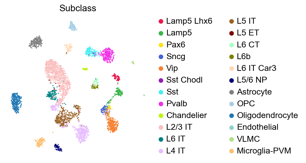
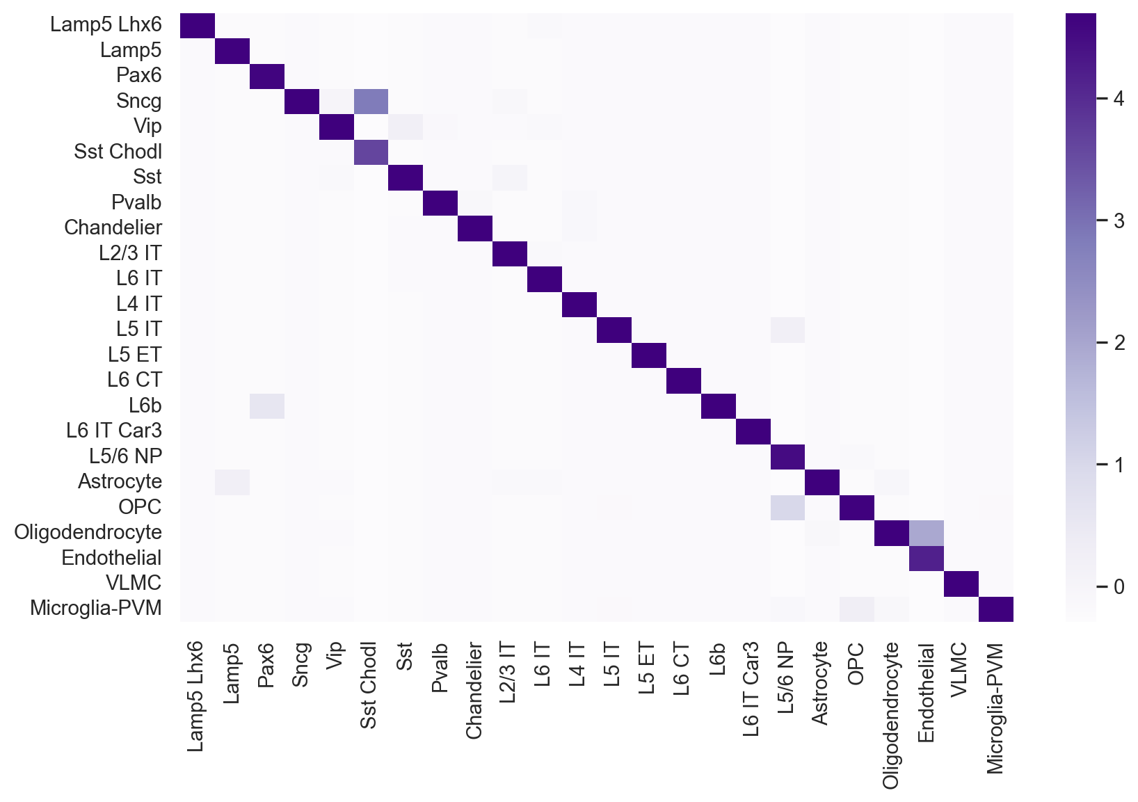
Since we know the real subclass of the test data, we can test the performance of predictCellTypeByGDR by comparing predicted celltypes and true subclasses.
[34]:
confusion_matrix = metrics.confusion_matrix(y[test_index], adata_test.obs['CellTypes_gdr'].values)
[35]:
confusion_matrix_df = pd.DataFrame(confusion_matrix, columns=adata_test.obs['Subclass'].cat.categories, index=adata_test.obs['Subclass'].cat.categories)
normalized_cf_matrix_df = (confusion_matrix_df - confusion_matrix_df.mean(axis=0))/confusion_matrix_df.std(axis=0)
[36]:
sns.set_style("whitegrid", {'axes.grid' : False})
sns.set(rc={'figure.figsize':(10, 6)})
sns.heatmap(normalized_cf_matrix_df,
            cmap="Purples",
            xticklabels=True,
            yticklabels=True)
plt.show()
[37]:
piaso_f1_score=np.round(f1_score(adata_test.obs['Subclass'], adata_test.obs['CellTypes_gdr'], average='micro'), decimals=3)
print(f"The Micro F1 score for PIASO prediction: {piaso_f1_score}")
piaso_f1_score=np.round(f1_score(adata_test.obs['Subclass'], adata_test.obs['CellTypes_gdr'], average='macro'), decimals=3)
print(f"The Macro F1 score for PIASO prediction: {piaso_f1_score}")
The Micro F1 score for PIASO prediction: 0.963
The Macro F1 score for PIASO prediction: 0.935