GDR: marker Gene-guided Dimensionality Reduction#
[1]:
import scanpy as sc
import os
from matplotlib import rcParams
import time
import warnings
[2]:
warnings.simplefilter(action='ignore', category=FutureWarning)
[3]:
path = '/home/vas744/Analysis/Python/Packages/PIASO'
import sys
sys.path.append(path)
path = '/home/vas744/Analysis/Python/Packages/COSG'
import sys
sys.path.append(path)
import piaso
import cosg
/home/vas744/.local/lib/python3.9/site-packages/networkx/utils/backends.py:135: RuntimeWarning: networkx backend defined more than once: nx-loopback
  backends.update(_get_backends("networkx.backends"))
[4]:
sc.set_figure_params(dpi=96,dpi_save=300, color_map='viridis',facecolor='white')
rcParams['figure.figsize'] = 4, 4
rcParams['font.sans-serif'] = "Arial"
rcParams['font.family'] = "Arial"
sc.settings.verbosity = 3
sc.logging.print_header()
scanpy==1.10.3 anndata==0.10.8 umap==0.5.7 numpy==1.26.4 scipy==1.13.0 pandas==2.2.3 scikit-learn==1.5.2 statsmodels==0.14.4 igraph==0.11.5 louvain==0.8.2 pynndescent==0.5.13
Load the data#
We will be using a Multiome RNA dataset obtained from cortex at P57.
Download the dataset from Google Drive: https://drive.google.com/file/d/1bEyWNjGvoA9kz3J6jnbXRKgAIytb555W/view?usp=drive_link
[5]:
!/home/vas744/Software/gdrive files download --overwrite --destination /n/scratch/users/v/vas744/Data/Public/PIASO 1bEyWNjGvoA9kz3J6jnbXRKgAIytb555W
Downloading AdultCortexMultiomeRNA_integrated_anno.h5ad
Successfully downloaded AdultCortexMultiomeRNA_integrated_anno.h5ad
[6]:
adata_path = os.path.join("/n/scratch/users/v/vas744/Data/Public/PIASO", "AdultCortexMultiomeRNA_integrated_anno.h5ad")
[7]:
adata = sc.read(
    adata_path,
)
adata
[7]:
AnnData object with n_obs × n_vars = 17412 × 26205
    obs: 'gex_barcode', 'atac_barcode', 'is_cell', 'excluded_reason', 'gex_raw_reads', 'gex_mapped_reads', 'gex_conf_intergenic_reads', 'gex_conf_exonic_reads', 'gex_conf_intronic_reads', 'gex_conf_exonic_unique_reads', 'gex_conf_exonic_antisense_reads', 'gex_conf_exonic_dup_reads', 'gex_exonic_umis', 'gex_conf_intronic_unique_reads', 'gex_conf_intronic_antisense_reads', 'gex_conf_intronic_dup_reads', 'gex_intronic_umis', 'gex_conf_txomic_unique_reads', 'gex_umis_count', 'gex_genes_count', 'atac_raw_reads', 'atac_unmapped_reads', 'atac_lowmapq', 'atac_dup_reads', 'atac_chimeric_reads', 'atac_mitochondrial_reads', 'atac_fragments', 'atac_TSS_fragments', 'atac_peak_region_fragments', 'atac_peak_region_cutsites', 'Sample', 'batch', 'n_genes', 'n_genes_by_counts', 'total_counts', 'total_counts_mt', 'pct_counts_mt', 'pct_counts_ribo', 'scrublet_score', 'predicted_doublets', 'scrublet_cluster_score', 'bh_pval', 'Leiden', 'Leiden_last', 'Leiden_last2', 'Leiden_sample', 'CellTypes_TACCO', 'Leiden_local', 'CellTypes'
    var: 'gene_ids', 'feature_types', 'genome', 'n_cells', 'mt', 'n_cells_by_counts', 'mean_counts', 'pct_dropout_by_counts', 'total_counts', 'means', 'variances', 'residual_variances', 'highly_variable_rank', 'highly_variable', 'highly_variable_nbatches', 'highly_variable_intersection'
    uns: 'CellTypes_TACCO_colors', 'CellTypes_colors', 'Leiden_colors', 'Leiden_last2_colors', 'Leiden_last_colors', 'Leiden_local_colors', 'Sample_colors', 'cosg', 'dendrogram_Leiden', 'dendrogram_Leiden_local', 'hvg', 'leiden', 'log1p', 'neighbors', 'umap'
    obsm: 'CellTypes_TACCO', 'X_pca', 'X_pca_harmony', 'X_umap', 'X_umap_pca', 'X_umap_raw'
    varm: 'CellTypes_TACCO'
    layers: 'log1p', 'raw'
    obsp: 'connectivities', 'distances'
[8]:
adata.X=adata.layers['log1p'].copy()
INFOG normalization#
[9]:
%%time
piaso.tl.infog(adata,
               layer='raw',
               n_top_genes=3000,)
The normalized data is saved as `infog` in `adata.layers`.
The highly variable genes are saved as `highly_variable` in `adata.var`.
Finished INFOG normalization.
CPU times: user 3.05 s, sys: 3.16 s, total: 6.21 s
Wall time: 6.2 s
Visualize with PCA-based UMAP#
First, we will use a standard PCA-based UMAP to visualize the batches and cell types in the dataset. This helps in assessing the presence of batch effects.
[10]:
sc.pp.neighbors(adata,
                use_rep='X_pca',
                n_neighbors=15,
                random_state=10,
                knn=True,
                method="umap")

sc.tl.umap(adata)

sc.pl.umap(adata,
           color=['Sample','CellTypes'],
           palette=piaso.pl.color.d_color4,
           cmap=piaso.pl.color.c_color4,
           size=10,
           ncols=1,
           frameon=False)
computing neighbors
    finished: added to `.uns['neighbors']`
    `.obsp['distances']`, distances for each pair of neighbors
    `.obsp['connectivities']`, weighted adjacency matrix (0:00:36)
computing UMAP
    finished: added
    'X_umap', UMAP coordinates (adata.obsm)
    'umap', UMAP parameters (adata.uns) (0:00:27)
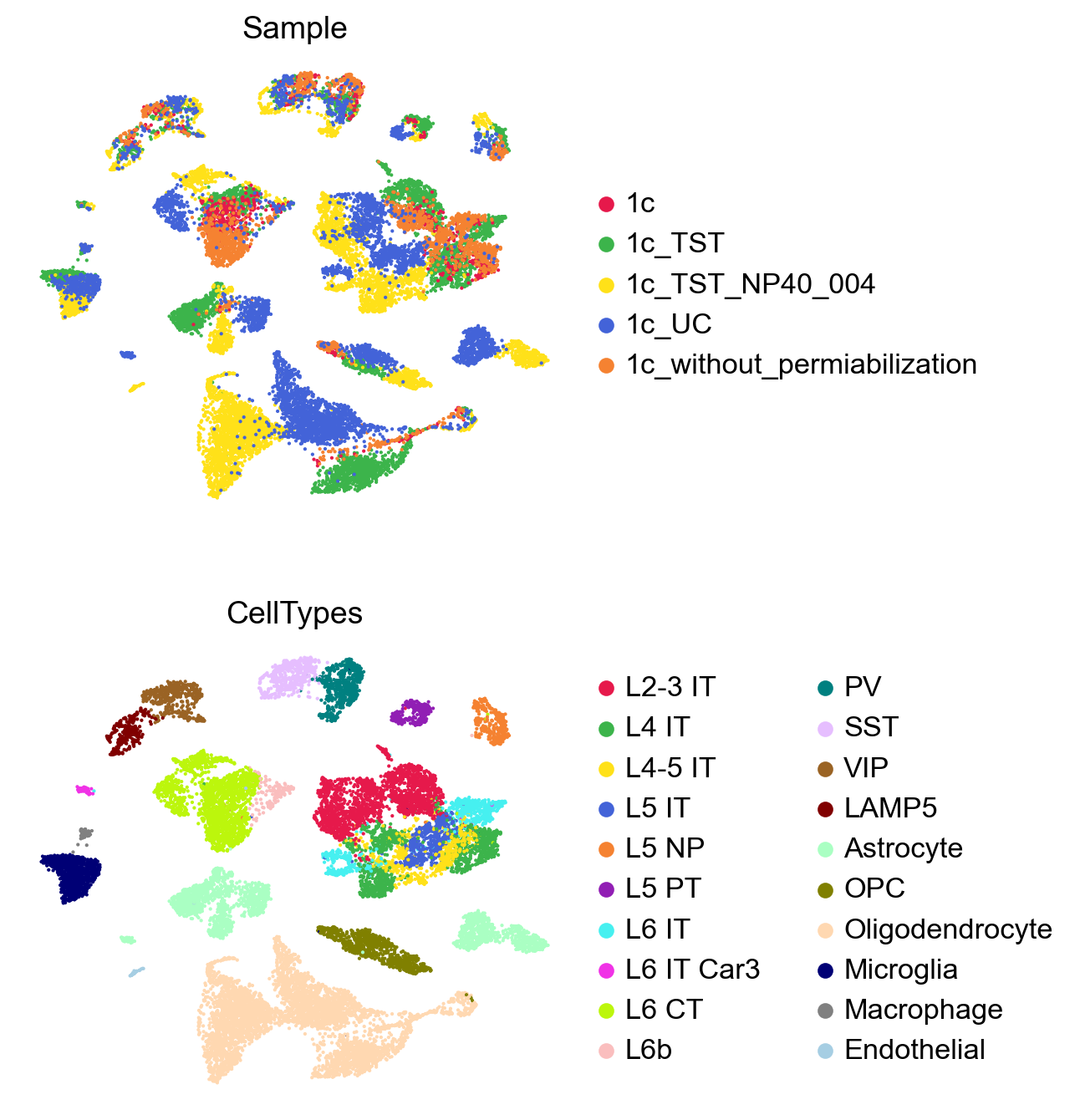
The UMAP plot clearly shows batch effects in the dataset.
Dimensionality reduction with GDRParallel#
In this turorial we will show how GDR works when only batch information is available and clusters or cell type informations isn’t available. In this case, runGDR clusters the data and infers the groups.
[11]:
%%time
piaso.tl.runGDRParallel(adata,
                        batch_key='Sample',
                        groupby=None,
                        n_gene=20,
                        mu=10,
                        resolution=3.0,
                        layer='infog',
                        infog_layer='raw',
                        score_layer='infog',
                        scoring_method='piaso',
                        use_highly_variable=True,
                        n_highly_variable_genes=5000,
                        n_svd_dims=50,
                        key_added='X_gdr',
                        max_workers=32,
                        calculate_score_multiBatch=False,
                        verbosity=0)
Calculating marker genes in batches: 100%|██████████| 5/5 [00:26<00:00,  5.38s/batch]
Calculating cell embeddings: 100%|██████████| 5/5 [00:59<00:00, 11.81s/batch]
The cell embeddings calculated by GDR were saved as `X_gdr` in adata.obsm.
CPU times: user 2.42 s, sys: 9.12 s, total: 11.5 s
Wall time: 1min 28s
Visualize GDR results with UMAPs#
[12]:
%%time
sc.pp.neighbors(adata,
                use_rep='X_gdr',
                n_neighbors=15,
                random_state=10,
                knn=True,
                method="umap")
sc.tl.umap(adata)
computing neighbors
    finished: added to `.uns['neighbors']`
    `.obsp['distances']`, distances for each pair of neighbors
    `.obsp['connectivities']`, weighted adjacency matrix (0:00:04)
computing UMAP
    finished: added
    'X_umap', UMAP coordinates (adata.obsm)
    'umap', UMAP parameters (adata.uns) (0:00:25)
CPU times: user 2min 16s, sys: 232 ms, total: 2min 17s
Wall time: 30.6 s
[13]:
sc.pl.umap(adata,
           color=['Sample','CellTypes'],
           palette=piaso.pl.color.d_color4,
           cmap=piaso.pl.color.c_color4,
           size=10,
           ncols=1,
           frameon=False)
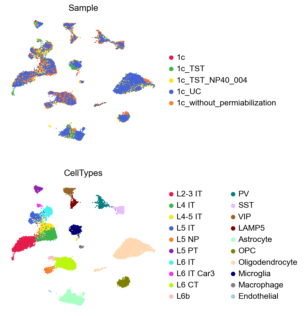
GDR effectively integrates batches and separates cell types using only dimensionality reduction, without additional integration methods.