Cell type prediction by GDR#
In this tutorial, we use a reference dataset to predict the cell type annotations of the query dataset. The cell type annotations of the query dataset are known, therefore our predictions can be verified and checked for accuracy.
[1]:
import numpy as np
import pandas as pd
import scanpy as sc
import matplotlib.pyplot as plt
from sklearn import metrics
import seaborn as sns
import logging
from matplotlib import rcParams
import sys
from sklearn.metrics import f1_score
import warnings
[2]:
warnings.simplefilter(action='ignore', category=FutureWarning)
[3]:
# To modify the default figure size, use rcParams.
sc.set_figure_params(dpi=80,dpi_save=300, color_map='viridis',facecolor='white')
rcParams['figure.figsize'] = 5, 5
rcParams['font.sans-serif'] = "Arial"
rcParams['font.family'] = "Arial"
sc.settings.verbosity = 3
sc.logging.print_header()
scanpy==1.10.3 anndata==0.10.8 umap==0.5.7 numpy==1.26.4 scipy==1.13.0 pandas==2.2.3 scikit-learn==1.5.2 statsmodels==0.14.4 igraph==0.11.5 louvain==0.8.2 pynndescent==0.5.13
[4]:
path = '/home/vas744/Analysis/Python/Packages/PIASO'
sys.path.append(path)
path = '/home/vas744/Analysis/Python/Packages/COSG'
sys.path.append(path)
import piaso
/home/vas744/.local/lib/python3.9/site-packages/networkx/utils/backends.py:135: RuntimeWarning: networkx backend defined more than once: nx-loopback
  backends.update(_get_backends("networkx.backends"))
Load the data#
Load the reference dataset#
We will use the 20k subsampled version of the Seattle Alzheimer’s Disease Brain Cell Atlas (SEA-AD) project dataset described in detail in Gabitto et. al. (2024), as the reference dataset. We will be using the scRNA-seq data from the dataset in this tutorial. Please refer to the Introduction tutorial to learn more about how it was preprocessed and normalized.
Download the subsampled, pre-processed dataset from Google Drive: https://drive.google.com/file/d/1pDBIgPvEO-sBuIMEhrvVhnf7tfU7H6Xy/view?usp=drive_link
The original data is available on https://portal.brain-map.org/explore/seattle-alzheimers-disease
[5]:
data_dir = "/n/scratch/users/v/vas744/Data/Public/PIASO"
[6]:
!/home/vas744/Software/gdrive files download --overwrite --destination {data_dir} 1pDBIgPvEO-sBuIMEhrvVhnf7tfU7H6Xy
Downloading SEA-AD_RNA_MTG_subsample_excludeReference_20k_piaso_preprocessed.h5ad
Successfully downloaded SEA-AD_RNA_MTG_subsample_excludeReference_20k_piaso_preprocessed.h5ad
[6]:
ref_adata=sc.read(data_dir + '/SEA-AD_RNA_MTG_subsample_excludeReference_20k_piaso_preprocessed.h5ad')

ref_adata
[6]:
AnnData object with n_obs × n_vars = 20000 × 36601
    obs: 'sample_id', 'Neurotypical reference', 'Donor ID', 'Organism', 'Brain Region', 'Sex', 'Gender', 'Age at Death', 'Race (choice=White)', 'Race (choice=Black/ African American)', 'Race (choice=Asian)', 'Race (choice=American Indian/ Alaska Native)', 'Race (choice=Native Hawaiian or Pacific Islander)', 'Race (choice=Unknown or unreported)', 'Race (choice=Other)', 'specify other race', 'Hispanic/Latino', 'Highest level of education', 'Years of education', 'PMI', 'Fresh Brain Weight', 'Brain pH', 'Overall AD neuropathological Change', 'Thal', 'Braak', 'CERAD score', 'Overall CAA Score', 'Highest Lewy Body Disease', 'Total Microinfarcts (not observed grossly)', 'Total microinfarcts in screening sections', 'Atherosclerosis', 'Arteriolosclerosis', 'LATE', 'Cognitive Status', 'Last CASI Score', 'Interval from last CASI in months', 'Last MMSE Score', 'Interval from last MMSE in months', 'Last MOCA Score', 'Interval from last MOCA in months', 'APOE Genotype', 'Primary Study Name', 'Secondary Study Name', 'NeuN positive fraction on FANS', 'RIN', 'cell_prep_type', 'facs_population_plan', 'rna_amplification', 'sample_name', 'sample_quantity_count', 'expc_cell_capture', 'method', 'pcr_cycles', 'percent_cdna_longer_than_400bp', 'rna_amplification_pass_fail', 'amplified_quantity_ng', 'load_name', 'library_prep', 'library_input_ng', 'r1_index', 'avg_size_bp', 'quantification_fmol', 'library_prep_pass_fail', 'exp_component_vendor_name', 'batch_vendor_name', 'experiment_component_failed', 'alignment', 'Genome', 'ar_id', 'bc', 'GEX_Estimated_number_of_cells', 'GEX_number_of_reads', 'GEX_sequencing_saturation', 'GEX_Mean_raw_reads_per_cell', 'GEX_Q30_bases_in_barcode', 'GEX_Q30_bases_in_read_2', 'GEX_Q30_bases_in_UMI', 'GEX_Percent_duplicates', 'GEX_Q30_bases_in_sample_index_i1', 'GEX_Q30_bases_in_sample_index_i2', 'GEX_Reads_with_TSO', 'GEX_Sequenced_read_pairs', 'GEX_Valid_UMIs', 'GEX_Valid_barcodes', 'GEX_Reads_mapped_to_genome', 'GEX_Reads_mapped_confidently_to_genome', 'GEX_Reads_mapped_confidently_to_intergenic_regions', 'GEX_Reads_mapped_confidently_to_intronic_regions', 'GEX_Reads_mapped_confidently_to_exonic_regions', 'GEX_Reads_mapped_confidently_to_transcriptome', 'GEX_Reads_mapped_antisense_to_gene', 'GEX_Fraction_of_transcriptomic_reads_in_cells', 'GEX_Total_genes_detected', 'GEX_Median_UMI_counts_per_cell', 'GEX_Median_genes_per_cell', 'Multiome_Feature_linkages_detected', 'Multiome_Linked_genes', 'Multiome_Linked_peaks', 'ATAC_Confidently_mapped_read_pairs', 'ATAC_Fraction_of_genome_in_peaks', 'ATAC_Fraction_of_high_quality_fragments_in_cells', 'ATAC_Fraction_of_high_quality_fragments_overlapping_TSS', 'ATAC_Fraction_of_high_quality_fragments_overlapping_peaks', 'ATAC_Fraction_of_transposition_events_in_peaks_in_cells', 'ATAC_Mean_raw_read_pairs_per_cell', 'ATAC_Median_high_quality_fragments_per_cell', 'ATAC_Non-nuclear_read_pairs', 'ATAC_Number_of_peaks', 'ATAC_Percent_duplicates', 'ATAC_Q30_bases_in_barcode', 'ATAC_Q30_bases_in_read_1', 'ATAC_Q30_bases_in_read_2', 'ATAC_Q30_bases_in_sample_index_i1', 'ATAC_Sequenced_read_pairs', 'ATAC_TSS_enrichment_score', 'ATAC_Unmapped_read_pairs', 'ATAC_Valid_barcodes', 'Number of mapped reads', 'Number of unmapped reads', 'Number of multimapped reads', 'Number of reads', 'Number of UMIs', 'Genes detected', 'Doublet score', 'Fraction mitochondrial UMIs', 'Used in analysis', 'Class confidence', 'Class', 'Subclass confidence', 'Subclass', 'Supertype confidence', 'Supertype (non-expanded)', 'Supertype', 'Continuous Pseudo-progression Score', 'Severely Affected Donor', 'n_genes', 'n_genes_by_counts', 'total_counts', 'total_counts_mt', 'pct_counts_mt', 'pct_counts_ribo'
    var: 'gene_ids', 'mt', 'n_cells_by_counts', 'mean_counts', 'pct_dropout_by_counts', 'total_counts', 'means', 'variances', 'residual_variances', 'highly_variable_rank', 'highly_variable'
    uns: 'APOE4 Status_colors', 'Braak_colors', 'CERAD score_colors', 'Cognitive Status_colors', 'Great Apes Metadata', 'Highest Lewy Body Disease_colors', 'LATE_colors', 'Overall AD neuropathological Change_colors', 'Sex_colors', 'Subclass_colors', 'Supertype_colors', 'Thal_colors', 'UW Clinical Metadata', 'X_normalization', 'batch_condition', 'default_embedding', 'hvg', 'log1p', 'neighbors', 'title', 'umap'
    obsm: 'X_scVI', 'X_svd', 'X_umap', 'X_umap_backup'
    layers: 'UMIs', 'log1p', 'raw'
    obsp: 'connectivities', 'distances'
Load the query dataset#
We will use a pre-processed Great Apes RNASeq data, particularly the human data subset as the query dataset for predicting cell types in this tutorial.
Download the dataset from: https://drive.google.com/file/d/1nF0iRTGFFQcEcM6hYcPptiYkxs65k2p4/view?usp=drive_link
[8]:
!/home/vas744/Software/gdrive files download --overwrite --destination {data_dir} 1nF0iRTGFFQcEcM6hYcPptiYkxs65k2p4
Downloading GreatApesMTG_RNA_integrated_raw_onlyOrthogonal_gdr_humanSubset_aibs.h5ad
Successfully downloaded GreatApesMTG_RNA_integrated_raw_onlyOrthogonal_gdr_humanSubset_aibs.h5ad
[7]:
aibs_query_adata = sc.read(data_dir + "/GreatApesMTG_RNA_integrated_raw_onlyOrthogonal_gdr_humanSubset_aibs.h5ad")
aibs_query_adata
[7]:
AnnData object with n_obs × n_vars = 76560 × 14346
    obs: 'nCount_RNA', 'nFeature_RNA', 'sample_id', 'dataset', 'donor', 'species', 'tech', 'species_tech', 'neighborhood', 'layer', 'cluster', 'cluster_color', 'cross_species_cluster', 'cross_species_cluster_color', 'sex', 'donor_color', 'subclass', 'subclass_color', 'class', 'UMAP_1', 'UMAP_2', 'batch', 'Sample', 'n_genes_by_counts', 'total_counts', 'total_counts_mt', 'pct_counts_mt', 'pct_counts_ribo', 'Leiden'
    var: 'mt', 'n_cells_by_counts', 'mean_counts', 'pct_dropout_by_counts', 'total_counts', 'means', 'variances', 'residual_variances', 'highly_variable_rank', 'highly_variable'
    uns: 'Leiden_colors', 'Sample_colors', 'hvg', 'leiden', 'log1p', 'neighbors', 'species_tech_colors', 'subclass_colors', 'umap'
    obsm: 'X_gdr', 'X_gdr_harmony', 'X_svd', 'X_umap', 'X_umap_gdr', 'X_umap_gdr_harmony', 'X_umap_published'
    layers: 'log1p', 'raw'
    obsp: 'connectivities', 'distances'
Visualize with UMAPs#
Reorder the query dataset categories to match the reference dataset categories
[8]:
categories = ['Astrocyte', 'Chandelier', 'Endothelial', 'L2/3 IT', 'L4 IT', 'L5 ET', 'L5 IT',
              'L5/6 NP', 'L6 CT', 'L6 IT', 'L6 IT Car3', 'L6b', 'Lamp5', 'Lamp5 Lhx6',
              'Microglia-PVM', 'OPC', 'Oligodendrocyte', 'Pax6', 'Pvalb', 'Sncg', 'Sst',
              'Sst Chodl', 'VLMC', 'Vip']
aibs_query_adata.obs['subclass'] = aibs_query_adata.obs['subclass'].cat.rename_categories(categories)
[9]:
aibs_query_adata.obs['subclass']=aibs_query_adata.obs['subclass'].astype('category')
aibs_query_adata.obs['subclass']=aibs_query_adata.obs['subclass'].cat.reorder_categories(ref_adata.obs['Subclass'].cat.categories)
[10]:
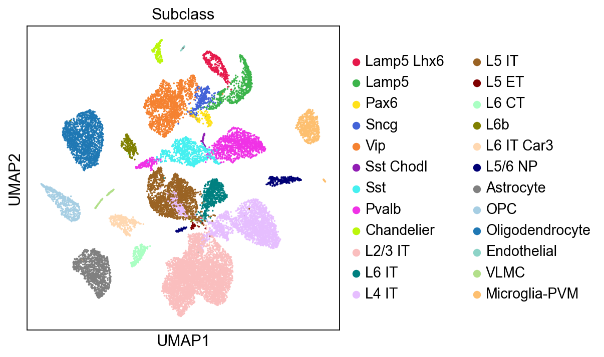
sc.pl.umap(ref_adata,
           color=['Subclass'],
           palette=piaso.pl.color.d_color4,
           ncols=1,
           size=10,
           frameon=True)
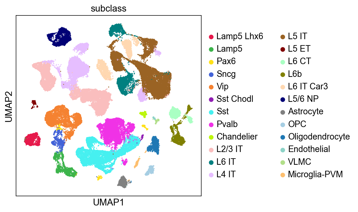
[11]:
sc.pl.umap(aibs_query_adata,
           color=['subclass'],
           palette=piaso.pl.color.d_color4,
           ncols=1,
           size=10,
           frameon=True)
Cluster the query data#
[12]:
%%time
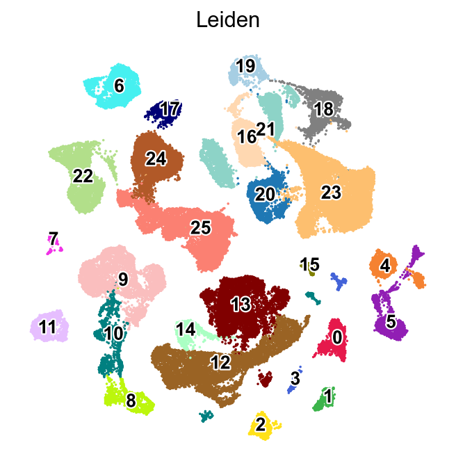
sc.tl.leiden(aibs_query_adata,resolution=0.2,key_added='Leiden',flavor="igraph",n_iterations=-1)
running Leiden clustering
    finished: found 26 clusters and added
    'Leiden', the cluster labels (adata.obs, categorical) (0:00:03)
CPU times: user 2.82 s, sys: 253 ms, total: 3.07 s
Wall time: 3.05 s
[13]:
logging.getLogger('matplotlib.font_manager').disabled = True
[14]:
sc.pl.umap(aibs_query_adata,
           color=['Leiden'],
           palette=piaso.pl.color.d_color4,
           legend_fontsize=12,
           legend_fontoutline=2,
           legend_loc='on data',
           ncols=1,
           size=10,
           frameon=False)
Predict cell types by GDR#
[15]:
piaso.tl.predictCellTypeByGDR(
    aibs_query_adata,
    ref_adata,
    layer = 'log1p',
    layer_reference = 'log1p',
    reference_groupby  = 'Subclass',
    query_groupby = 'Leiden',
    mu = 10.0,
    n_genes= 15,
    return_integration = False,
    use_highly_variable = True,
    n_highly_variable_genes = 5000,
    n_svd_dims = 50,
    resolution= 1.0,
    scoring_method= None,
    key_added= None,
    verbosity= 0,
)
Running GDR for the query dataset and the reference dataset:
GDR embeddings saved to adata.obsm['X_gdr']
2025-03-13 17:56:06,884 - harmonypy - INFO - Computing initial centroids with sklearn.KMeans...
2025-03-13 17:56:17,410 - harmonypy - INFO - sklearn.KMeans initialization complete.
2025-03-13 17:56:18,858 - harmonypy - INFO - Iteration 1 of 10
2025-03-13 17:57:19,554 - harmonypy - INFO - Iteration 2 of 10
2025-03-13 17:58:25,833 - harmonypy - INFO - Iteration 3 of 10
2025-03-13 17:58:58,705 - harmonypy - INFO - Iteration 4 of 10
2025-03-13 17:59:24,916 - harmonypy - INFO - Iteration 5 of 10
2025-03-13 17:59:46,990 - harmonypy - INFO - Converged after 5 iterations
Predicting cell types:
All finished. The predicted cell types are saved as `CellTypes_gdr` in adata.obs.
Reorder the query dataset categories to match the reference dataset categories
[16]:
aibs_query_adata.obs['CellTypes_gdr']=aibs_query_adata.obs['CellTypes_gdr'].astype('category')
aibs_query_adata.obs['CellTypes_gdr']=aibs_query_adata.obs['CellTypes_gdr'].cat.reorder_categories(aibs_query_adata.obs['subclass'].cat.categories)
We can now visualize the predicted cell types from GDR using a UMAP and compare them with the UMAP of the true cell types.
[17]:
sc.pl.embedding(aibs_query_adata,
                basis='X_umap',
                color=['CellTypes_gdr', 'subclass'],
                palette=piaso.pl.color.d_color4,
                cmap=piaso.pl.color.c_color3,
                ncols=1,
                size=10,
                frameon=False)
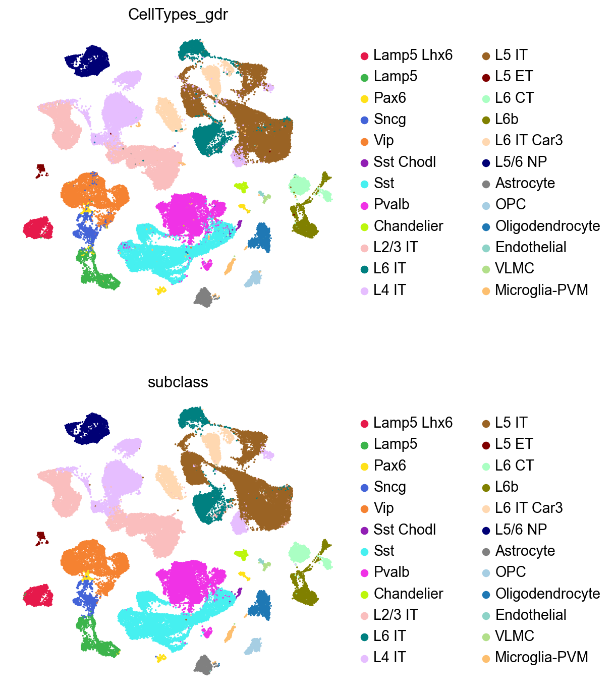
Since we know the real subclass of the test data, we can test the performance of predictCellTypeByGDR by comparing predicted celltypes and true subclasses.
[18]:
confusion_matrix = metrics.confusion_matrix(aibs_query_adata.obs['subclass'].values, aibs_query_adata.obs['CellTypes_gdr'].values)
confusion_matrix_df = pd.DataFrame(confusion_matrix, columns=aibs_query_adata.obs['subclass'].cat.categories, index=aibs_query_adata.obs['subclass'].cat.categories)
[19]:
normalized_cf_matrix_df = confusion_matrix_df/confusion_matrix_df.sum(axis=0)
[20]:
sns.set_style("whitegrid", {'axes.grid' : False})
sns.set(rc={'figure.figsize':(8, 6)})
sns.heatmap(normalized_cf_matrix_df,
            cmap="Purples",
            xticklabels=True,
            yticklabels=True)
plt.xlabel("Predicted Subclass")
plt.ylabel("True Subclass")
plt.show()
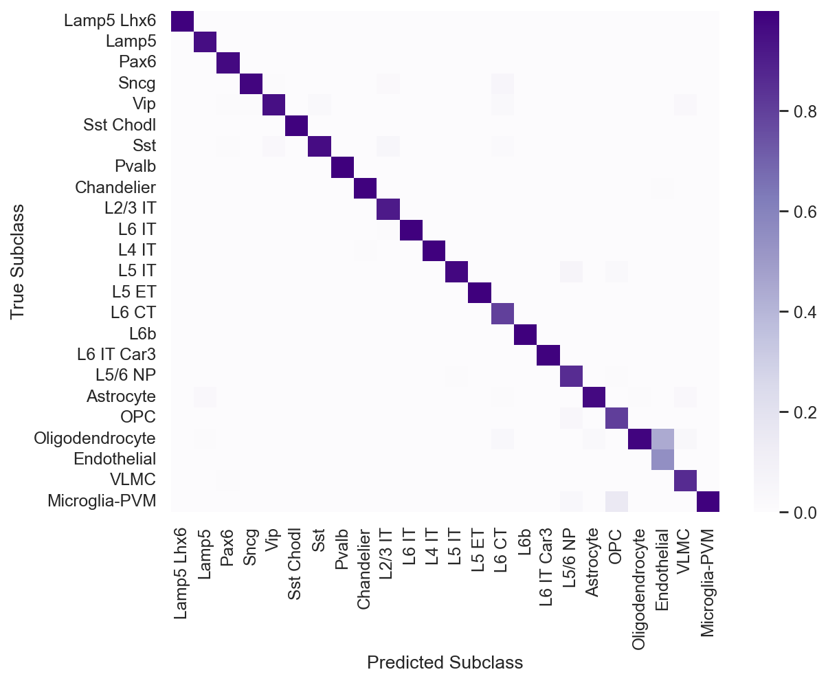
[21]:
piaso_f1_score=np.round(f1_score(aibs_query_adata.obs['subclass'], aibs_query_adata.obs['CellTypes_gdr'], average='micro'), decimals=3)
print(f"The Micro F1 score for PIASO prediction: {piaso_f1_score}")
piaso_f1_score=np.round(f1_score(aibs_query_adata.obs['subclass'], aibs_query_adata.obs['CellTypes_gdr'], average='macro'), decimals=3)
print(f"The Macro F1 score for PIASO prediction: {piaso_f1_score}")
The Micro F1 score for PIASO prediction: 0.967
The Macro F1 score for PIASO prediction: 0.951