Pre-processing CellRanger outputs (single sample, Human PBMCs)#
This notebook demonstrates the pipeline for processing scRNA-seq data, covering metric computation, normalization, clustering, cell type prediction, and the identification/removal of doublets and low-quality clusters. The final output is pre-processed, annotated scRNA-seq data.
[1]:
import piaso
import cosg
import numpy as np
import pandas as pd
import scanpy as sc
import logging
from sklearn.preprocessing import StandardScaler
import warnings

from matplotlib import rcParams
sc.settings.set_figure_params(scanpy=True, dpi=80, dpi_save=300, frameon=True, vector_friendly=False, fontsize=14)
import matplotlib as mpl
mpl.rcParams['pdf.fonttype'] = 42
mpl.rcParams['ps.fonttype'] = 42
/n/data1/hms/neurobio/fishell/vallaris/.conda/envs/piaso_env/lib/python3.10/site-packages/tqdm/auto.py:21: TqdmWarning: IProgress not found. Please update jupyter and ipywidgets. See https://ipywidgets.readthedocs.io/en/stable/user_install.html
  from .autonotebook import tqdm as notebook_tqdm
[2]:
data_dir = "/n/scratch/users/v/vas744/Data/Public/PBMCMultiomeRop2023"
save_dir = "/n/scratch/users/v/vas744/Results/single-cell/Methods/DataProcessing/PBMCMultiomeRop2023"
prefix = "HumanPBMCs_Multiome_RNA"
Download the data#
Human PBMC snMultiome data (SAN2) from: De Rop, F.V., Hulselmans, G., Flerin, C. et al. Systematic benchmarking of single-cell ATAC-sequencing protocols. Nat Biotechnol 42, 916–926 (2024). https://doi.org/10.1038/s41587-023-01881-x
Also available via https://drive.google.com/file/d/1g1V-VTy2qHK7PJIbW-t9hRFzHCqFCe4T/view?usp=drive_link
[3]:
# !/home/vas744/Software/gdrive files download --destination /n/scratch/users/v/vas744/Data/Public/PBMCMultiomeRop2023 1g1V-VTy2qHK7PJIbW-t9hRFzHCqFCe4T
Load the data#
[4]:
data_path = data_dir + "/filtered_feature_bc_matrix.h5"
adata=sc.read_10x_h5(data_path)
adata
/n/data1/hms/neurobio/fishell/vallaris/.conda/envs/piaso_env/lib/python3.10/site-packages/anndata/_core/anndata.py:1758: UserWarning: Variable names are not unique. To make them unique, call `.var_names_make_unique`.
  utils.warn_names_duplicates("var")
/n/data1/hms/neurobio/fishell/vallaris/.conda/envs/piaso_env/lib/python3.10/site-packages/anndata/_core/anndata.py:1758: UserWarning: Variable names are not unique. To make them unique, call `.var_names_make_unique`.
  utils.warn_names_duplicates("var")
[4]:
AnnData object with n_obs × n_vars = 4360 × 36601
    var: 'gene_ids', 'feature_types', 'genome', 'interval'
[5]:
adata.var_names_make_unique()
This dataset contains a single sample, but we will add a Sample column to adata.obs and assign a sample name to facilitate downstream analysis.
[6]:
adata.obs['Sample']="Human_PBMCs"
[7]:
adata.X.data
[7]:
array([ 2., 1., 1., ..., 43., 18., 56.], shape=(6669764,), dtype=float32)
Create the ‘raw’ counts layer based on the counts data from the adata object.
[8]:
adata.layers['raw'] = adata.X
adata
[8]:
AnnData object with n_obs × n_vars = 4360 × 36601
    obs: 'Sample'
    var: 'gene_ids', 'feature_types', 'genome', 'interval'
    layers: 'raw'
[9]:
adata.var
[9]:
| gene_ids | feature_types | genome | interval | |
|---|---|---|---|---|
| MIR1302-2HG | ENSG00000243485 | Gene Expression | GRCh38 | chr1:29553-30267 |
| FAM138A | ENSG00000237613 | Gene Expression | GRCh38 | chr1:36080-36081 |
| OR4F5 | ENSG00000186092 | Gene Expression | GRCh38 | chr1:65418-69055 |
| AL627309.1 | ENSG00000238009 | Gene Expression | GRCh38 | chr1:120931-133723 |
| AL627309.3 | ENSG00000239945 | Gene Expression | GRCh38 | chr1:91104-91105 |
| ... | ... | ... | ... | ... |
| AC141272.1 | ENSG00000277836 | Gene Expression | GRCh38 | KI270728.1:1270983-1270984 |
| AC023491.2 | ENSG00000278633 | Gene Expression | GRCh38 | KI270731.1:13000-13001 |
| AC007325.1 | ENSG00000276017 | Gene Expression | GRCh38 | KI270734.1:72410-72411 |
| AC007325.4 | ENSG00000278817 | Gene Expression | GRCh38 | KI270734.1:131493-131494 |
| AC007325.2 | ENSG00000277196 | Gene Expression | GRCh38 | KI270734.1:161749-161852 |
36601 rows × 4 columns
Quality Control#
Filter cells based on gene counts#
Filter out cells with fewer than 200 detected genes.
[10]:
sc.pp.filter_cells(adata, min_genes=200)
Calculate cell quality metrics#
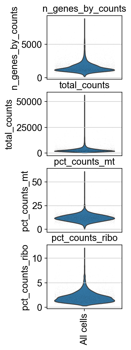
We identify mitochondrial and ribosomal protein genes and compute their proportion in each cell’s total read count. A high proportion of these reads often indicates low-quality cells. Note: In human data, the gene names have uppercase letters (MT-, RPS-, RPL-). For mouse data, these gene names will start with Mt-, Rps-, Rpl-
[11]:
adata.var['mt'] = adata.var_names.str.startswith('MT-')
sc.pp.calculate_qc_metrics(adata, qc_vars=['mt'], percent_top=None, log1p=False, inplace=True)
[12]:
adata.var['ribo'] = adata.var_names.str.startswith('RPS','RPL')
sc.pp.calculate_qc_metrics(adata, qc_vars=['ribo'], percent_top=None, log1p=False, inplace=True)
/tmp/ipykernel_842045/3834852883.py:1: FutureWarning: Allowing a non-bool 'na' in obj.str.startswith is deprecated and will raise in a future version.
  adata.var['ribo'] = adata.var_names.str.startswith('RPS','RPL')
[13]:
piaso.pl.plot_features_violin(adata,
                              ['n_genes_by_counts', 'total_counts', 'pct_counts_mt','pct_counts_ribo'],
                              width_single=2.0)
Doublet prediction#
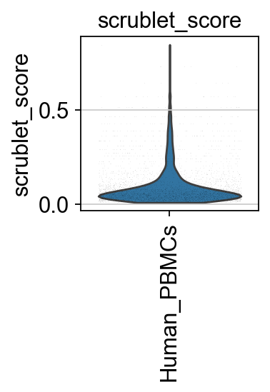
Next, we compute the scrublet score to identify and predict potential doublets.
[14]:
experiments=np.unique(adata.obs['Sample'])
adata.obs['scrublet_score']=np.repeat(0,adata.n_obs)
adata.obs['predicted_doublets']=np.repeat(False,adata.n_obs)
[15]:
import scrublet as scr

for experiment in experiments:
    print(experiment)
    adatai=adata[adata.obs['Sample']==experiment]

    scrub = scr.Scrublet(adatai.X.todense(),random_state=10)
    doublet_scores, predicted_doublets = scrub.scrub_doublets()

    adata.obs['predicted_doublets'][adatai.obs_names]=predicted_doublets

    adata.obs['scrublet_score'][adatai.obs_names]=doublet_scores
Human_PBMCs
Preprocessing...
Simulating doublets...
Embedding transcriptomes using PCA...
Calculating doublet scores...
Automatically set threshold at doublet score = 0.14
Detected doublet rate = 17.0%
Estimated detectable doublet fraction = 79.6%
Overall doublet rate:
        Expected   = 10.0%
        Estimated  = 21.4%
Elapsed time: 7.3 seconds
/tmp/ipykernel_842045/3464195482.py:10: FutureWarning: ChainedAssignmentError: behaviour will change in pandas 3.0!
You are setting values through chained assignment. Currently this works in certain cases, but when using Copy-on-Write (which will become the default behaviour in pandas 3.0) this will never work to update the original DataFrame or Series, because the intermediate object on which we are setting values will behave as a copy.
A typical example is when you are setting values in a column of a DataFrame, like:

df["col"][row_indexer] = value

Use `df.loc[row_indexer, "col"] = values` instead, to perform the assignment in a single step and ensure this keeps updating the original `df`.

See the caveats in the documentation: https://pandas.pydata.org/pandas-docs/stable/user_guide/indexing.html#returning-a-view-versus-a-copy

  adata.obs['predicted_doublets'][adatai.obs_names]=predicted_doublets
/tmp/ipykernel_842045/3464195482.py:10: SettingWithCopyWarning:
A value is trying to be set on a copy of a slice from a DataFrame

See the caveats in the documentation: https://pandas.pydata.org/pandas-docs/stable/user_guide/indexing.html#returning-a-view-versus-a-copy
  adata.obs['predicted_doublets'][adatai.obs_names]=predicted_doublets
/tmp/ipykernel_842045/3464195482.py:12: FutureWarning: ChainedAssignmentError: behaviour will change in pandas 3.0!
You are setting values through chained assignment. Currently this works in certain cases, but when using Copy-on-Write (which will become the default behaviour in pandas 3.0) this will never work to update the original DataFrame or Series, because the intermediate object on which we are setting values will behave as a copy.
A typical example is when you are setting values in a column of a DataFrame, like:

df["col"][row_indexer] = value

Use `df.loc[row_indexer, "col"] = values` instead, to perform the assignment in a single step and ensure this keeps updating the original `df`.

See the caveats in the documentation: https://pandas.pydata.org/pandas-docs/stable/user_guide/indexing.html#returning-a-view-versus-a-copy

  adata.obs['scrublet_score'][adatai.obs_names]=doublet_scores
/tmp/ipykernel_842045/3464195482.py:12: SettingWithCopyWarning:
A value is trying to be set on a copy of a slice from a DataFrame

See the caveats in the documentation: https://pandas.pydata.org/pandas-docs/stable/user_guide/indexing.html#returning-a-view-versus-a-copy
  adata.obs['scrublet_score'][adatai.obs_names]=doublet_scores
/tmp/ipykernel_842045/3464195482.py:12: FutureWarning: Setting an item of incompatible dtype is deprecated and will raise an error in a future version of pandas. Value '[0.07518797 0.29180328 0.03955842 ... 0.13812155 0.07239264 0.06466513]' has dtype incompatible with int64, please explicitly cast to a compatible dtype first.
  adata.obs['scrublet_score'][adatai.obs_names]=doublet_scores
[16]:
piaso.pl.plot_features_violin(adata,
                              ['scrublet_score'],
                              groupby='Sample',
                              width_single=2)
log1p Normalization#
[17]:
%%time
sc.pp.normalize_total(adata, target_sum=1e4)
sc.pp.log1p(adata)

adata.layers['log1p']=adata.X.copy()
CPU times: user 159 ms, sys: 14.2 ms, total: 173 ms
Wall time: 143 ms
INFOG Normalization#
We use PIASO’s INFOG to normalize the data and identify a highly variable set of genes.
[18]:
%%time
piaso.tl.infog(adata,
               copy=False,
               inplace=False,
               n_top_genes=3000,
               key_added='infog',
               key_added_highly_variable_gene='highly_variable',
               layer='raw')
The normalized data is saved as `infog` in `adata.layers`.
The highly variable genes are saved as `highly_variable` in `adata.var`.
Finished INFOG normalization.
CPU times: user 434 ms, sys: 78.8 ms, total: 513 ms
Wall time: 513 ms
Dimensionality reduction#
[19]:
%%time
piaso.tl.runSVD(adata,
                use_highly_variable=True,
                n_components=30,
                random_state=10,
                key_added='X_svd',
                layer='infog')
CPU times: user 2.95 s, sys: 3.4 ms, total: 2.95 s
Wall time: 477 ms
[20]:
%%time
sc.pp.neighbors(adata,
                use_rep='X_svd',
                n_neighbors=15,
                random_state=10,
                knn=True,
                method="umap")

sc.tl.umap(adata)
CPU times: user 26.6 s, sys: 107 ms, total: 26.7 s
Wall time: 24.5 s
[21]:
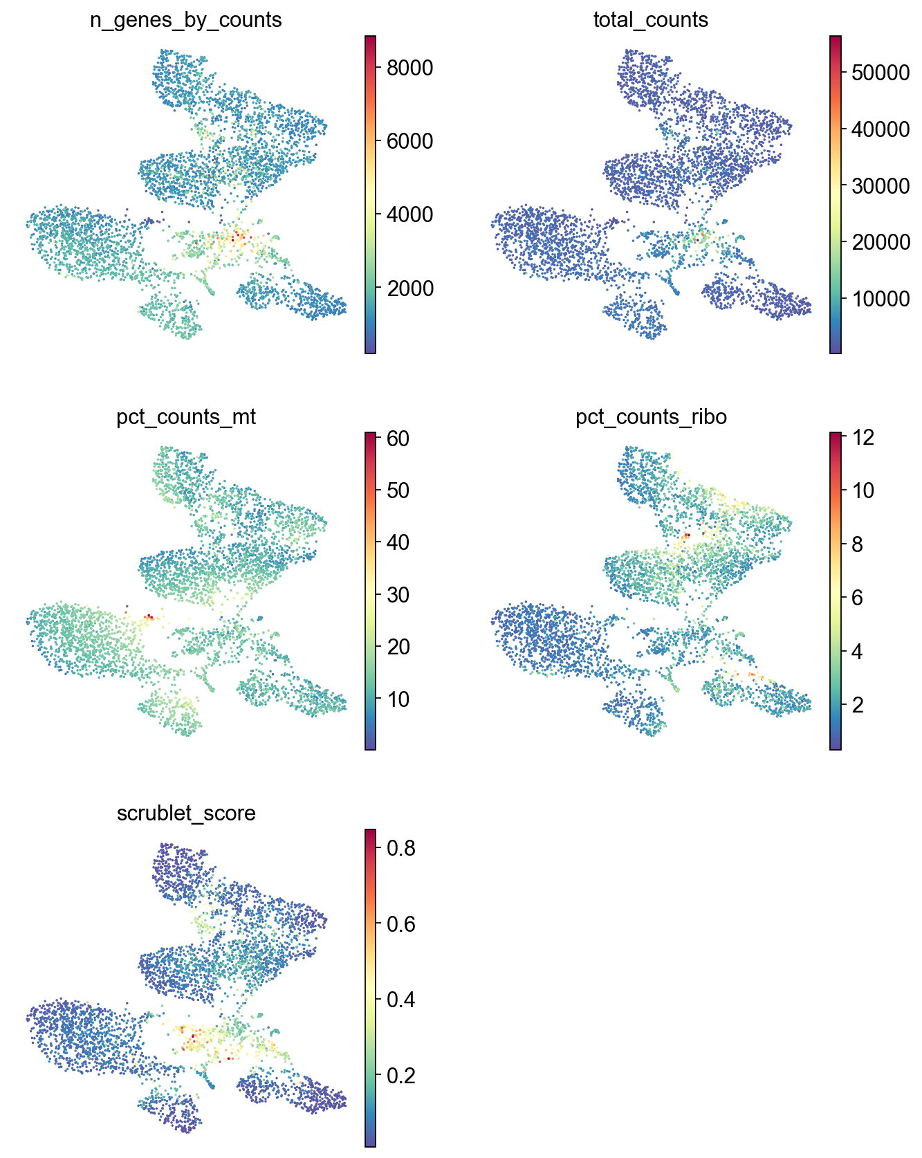
sc.pl.umap(adata,
           color=['n_genes_by_counts', 'total_counts','pct_counts_mt','pct_counts_ribo', 'scrublet_score'],
           cmap='Spectral_r',
           palette=piaso.pl.color.d_color1,
           ncols=2,
           size=10,
           frameon=False)
Save the data#
[22]:
save_dir+'/'+prefix+'_raw_QC.h5ad'
[22]:
'/n/scratch/users/v/vas744/Results/single-cell/Methods/DataProcessing/PBMCMultiomeRop2023/HumanPBMCs_Multiome_RNA_raw_QC.h5ad'
[23]:
adata.write(save_dir+'/'+prefix+'_raw_QC.h5ad')
[24]:
# adata = sc.read(save_dir+'/'+prefix+'_raw_QC.h5ad')
Filtering cells#
Outlier cells of these thresholds are likely low quality cells, so we filter them out before further downstream analysis.
[25]:
adata=adata[adata.obs['n_genes_by_counts']>500].copy()
[26]:
adata=adata[adata.obs['n_genes_by_counts']<10000].copy()
Remove doublets based on a scrublet score threshold.
[27]:
adata = adata[adata.obs['scrublet_score']<0.3].copy()
adata
[27]:
AnnData object with n_obs × n_vars = 3988 × 36601
    obs: 'Sample', 'n_genes', 'n_genes_by_counts', 'total_counts', 'total_counts_mt', 'pct_counts_mt', 'total_counts_ribo', 'pct_counts_ribo', 'scrublet_score', 'predicted_doublets'
    var: 'gene_ids', 'feature_types', 'genome', 'interval', 'mt', 'n_cells_by_counts', 'mean_counts', 'pct_dropout_by_counts', 'total_counts', 'ribo', 'infog_var', 'highly_variable'
    uns: 'Sample_colors', 'log1p', 'neighbors', 'umap'
    obsm: 'X_svd', 'X_umap'
    layers: 'raw', 'log1p', 'infog'
    obsp: 'distances', 'connectivities'
[28]:
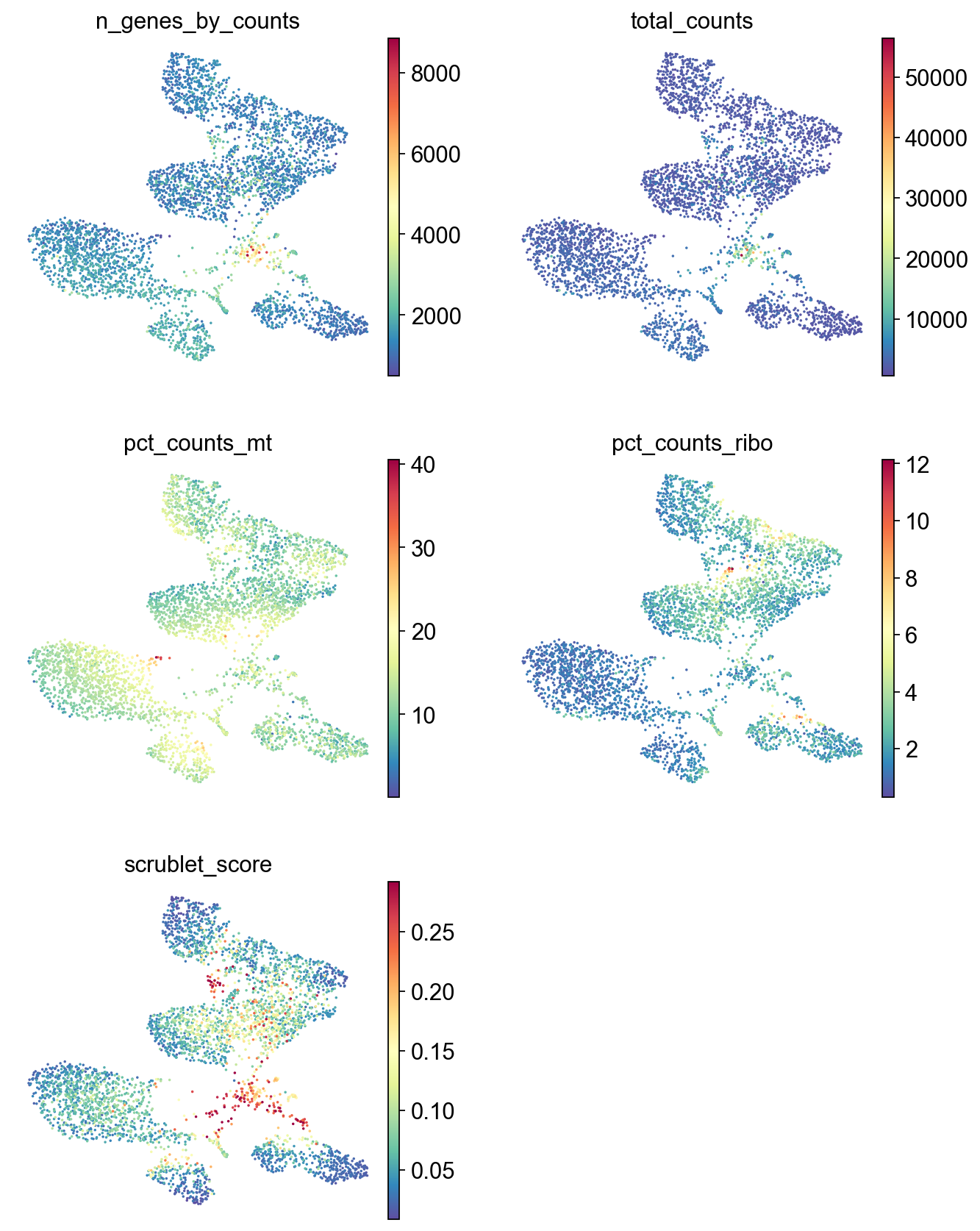
sc.pl.umap(adata,
           color=['n_genes_by_counts', 'total_counts','pct_counts_mt','pct_counts_ribo', 'scrublet_score'],
           cmap='Spectral_r',
           palette=piaso.pl.color.d_color1,
           ncols=2,
           size=10,
           frameon=False)
Annotation#
We used the precomputed Human PBMC marker gene sets from the AllenHumanImmuneHealthAtlas_L2 study in PIASOmarkerDB. The original dataset comes from https://www.nature.com/articles/s41586-025-09686-5.
[29]:
marker_gene_df = pd.read_csv("/n/scratch/users/v/vas744/Data/Public/10x_Human_PBMC/PIASOmarkerDB_AllenHumanImmuneHealthAtlas_L2_251219.csv")
marker_gene_df
[29]:
| Cell_Type | Gene | Specificity_Score | Study_Publication | Species | Tissue | Condition | |
|---|---|---|---|---|---|---|---|
| 0 | Platelet | GP9 | 16.455748 | AllenHumanImmuneHealthAtlas_L2 | Human | blood | normal |
| 1 | Erythrocyte | ALAS2 | 16.422475 | AllenHumanImmuneHealthAtlas_L2 | Human | blood | normal |
| 2 | Platelet | CMTM5 | 16.400534 | AllenHumanImmuneHealthAtlas_L2 | Human | blood | normal |
| 3 | Platelet | TMEM40 | 16.373334 | AllenHumanImmuneHealthAtlas_L2 | Human | blood | normal |
| 4 | Erythrocyte | AHSP | 16.338337 | AllenHumanImmuneHealthAtlas_L2 | Human | blood | normal |
| ... | ... | ... | ... | ... | ... | ... | ... |
| 1445 | Memory CD4 T cell | FXYD7 | 1.783520 | AllenHumanImmuneHealthAtlas_L2 | Human | blood | normal |
| 1446 | Memory CD4 T cell | CRIP1 | 1.779265 | AllenHumanImmuneHealthAtlas_L2 | Human | blood | normal |
| 1447 | Memory CD4 T cell | CCDC167 | 1.775660 | AllenHumanImmuneHealthAtlas_L2 | Human | blood | normal |
| 1448 | Memory CD4 T cell | CD6 | 1.775110 | AllenHumanImmuneHealthAtlas_L2 | Human | blood | normal |
| 1449 | Memory CD4 T cell | TMEM238 | 1.769377 | AllenHumanImmuneHealthAtlas_L2 | Human | blood | normal |
1450 rows × 7 columns
Preprocessing cell type-specific marker gene sets#
PIASO’s predictCellTypeByMarker expects the marker_gene_list in DataFrame or dict format. So here, we will create a dictionary with each cell type and their respective marker gene lists.
[30]:
marker_gene_dict = {}
cell_types = np.unique(marker_gene_df['Cell_Type'])
for cell_type in cell_types:
    marker_gene_dict[cell_type] = list(marker_gene_df[marker_gene_df['Cell_Type']==cell_type]['Gene'])
1. INFOG Normalization#
[31]:
%%time
piaso.tl.infog(adata,
               copy=False,
               inplace=False,
               n_top_genes=3000,
               key_added='infog',
               key_added_highly_variable_gene='highly_variable',
               layer='raw')
The normalized data is saved as `infog` in `adata.layers`.
The highly variable genes are saved as `highly_variable` in `adata.var`.
Finished INFOG normalization.
CPU times: user 367 ms, sys: 2.83 ms, total: 369 ms
Wall time: 370 ms
Dimensionality reduction#
[32]:
%%time
piaso.tl.runSVD(adata,
                use_highly_variable=True,
                n_components=30,
                random_state=10,
                key_added='X_svd',
                layer='infog')
CPU times: user 1.76 s, sys: 1.68 ms, total: 1.76 s
Wall time: 395 ms
[33]:
%%time
sc.pp.neighbors(adata,
                use_rep='X_svd',
                n_neighbors=15,
                random_state=10,
                knn=True,
                method="umap")

sc.tl.umap(adata)
CPU times: user 17.6 s, sys: 2.34 ms, total: 17.6 s
Wall time: 14.4 s
Predict cell types based on marker gene sets#
Here, we use the use_score = False to make the predictions based on p-values, but you can also use the gene set scores with use_score = True.
[34]:
%%time
piaso.tl.predictCellTypeByMarker(adata,
                                 marker_gene_set=marker_gene_dict,
                                 score_method='piaso',
                                 use_rep='X_svd',
                                 use_score=False,
                                 smooth_prediction=True,
                                 inplace=True)
Calculating gene set scores using piaso method...
Scoring gene sets: 100%|██████████| 29/29 [00:16<00:00, 1.72set/s]
Predicting cell types based on marker gene p-values...
Smoothing cell type predictions...
Smoothing cell type predictions from 'CellTypes_predicted_raw' using 7-nearest neighbors
Smoothed predictions stored in adata.obs['CellTypes_predicted_smoothed']
Confidence scores stored in adata.obs['CellTypes_predicted_smoothed_confidence']
Modified 934 cell labels (23.42% of total)
Cell type prediction completed. Results saved to:
  - adata.obs['CellTypes_predicted']: predicted cell types
  - adata.obsm['CellTypes_predicted_score']: full score matrix
  - adata.obsm['CellTypes_predicted_nlog10pvals']: full -log10(p-value) matrix
  - adata.obs['CellTypes_predicted_nlog10pvals']: maximum -log10(p-values)
  - adata.obs['CellTypes_predicted_raw']: original unsmoothed predictions
  - adata.obs['CellTypes_predicted_confidence_smoothed']: smoothing confidence scores
CPU times: user 3.78 s, sys: 91.7 ms, total: 3.87 s
Wall time: 22 s
[35]:
sc.pl.umap(adata,
color=['CellTypes_predicted'],
palette=piaso.pl.color.d_color20,
legend_fontsize=8,
legend_fontoutline=1,
# legend_loc='on data',
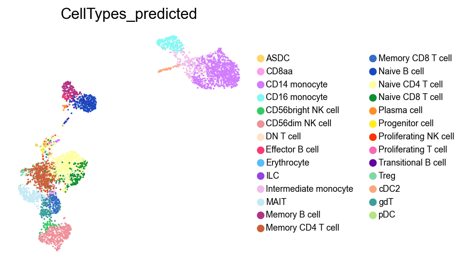
ncols=1,
size=10,
frameon=False)
Clustering#
[36]:
%%time
sc.tl.leiden(adata,resolution=2.5,key_added='Leiden')
<timed eval>:1: FutureWarning: In the future, the default backend for leiden will be igraph instead of leidenalg.

 To achieve the future defaults please pass: flavor="igraph" and n_iterations=2.  directed must also be False to work with igraph's implementation.
CPU times: user 1.77 s, sys: 1.04 ms, total: 1.77 s
Wall time: 1.77 s
[37]:
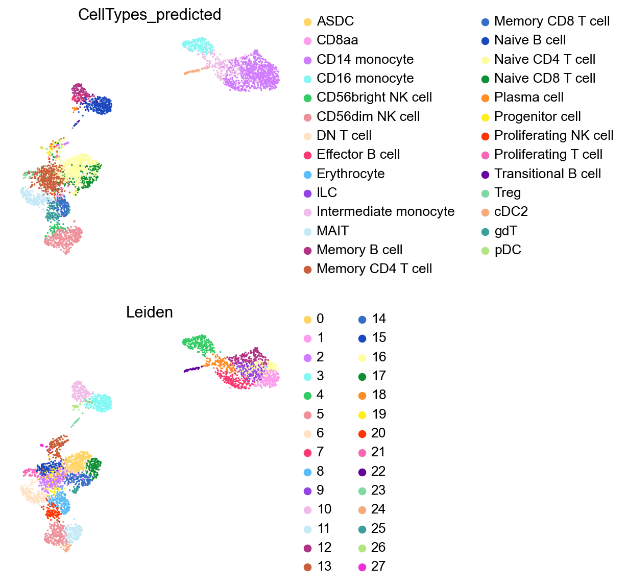
sc.pl.umap(adata,
           color=['CellTypes_predicted','Leiden'],
           palette=piaso.pl.color.d_color20,
           legend_fontsize=12,
           legend_fontoutline=2,
           # legend_loc='on data',
           ncols=1,
           size=10,
           frameon=False)
Identify marker genes with COSG#
[38]:
%%time
n_gene=30
cosg.cosg(adata,
          key_added='cosg',
          use_raw=False,
          layer='infog',
          mu=100,
          expressed_pct=0.1,
          remove_lowly_expressed=True,
          n_genes_user=n_gene,
          groupby='Leiden')
CPU times: user 577 ms, sys: 1.92 ms, total: 579 ms
Wall time: 580 ms
[39]:
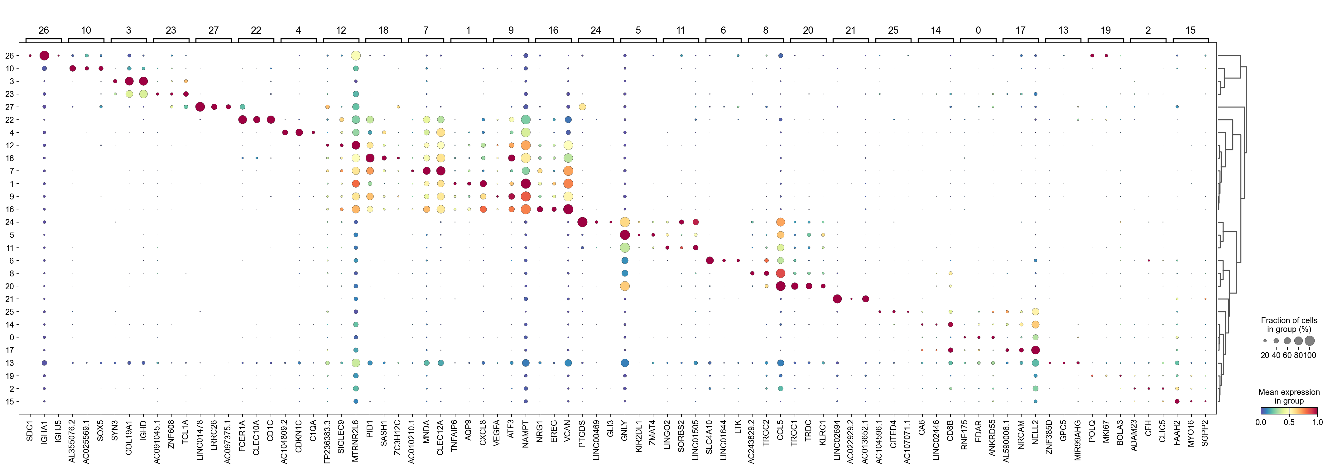
sc.tl.dendrogram(adata,groupby='Leiden',use_rep='X_svd')
df_tmp=pd.DataFrame(adata.uns['cosg']['names'][:3,]).T
df_tmp=df_tmp.reindex(adata.uns['dendrogram_'+'Leiden']['categories_ordered'])
marker_genes_list={idx: list(row.values) for idx, row in df_tmp.iterrows()}
marker_genes_list = {k: v for k, v in marker_genes_list.items() if not any(isinstance(x, float) for x in v)}

sc.pl.dotplot(adata,
              marker_genes_list,
              groupby='Leiden',
              layer='infog',
              dendrogram=True,
              swap_axes=False,
              standard_scale='var',
              cmap='Spectral_r')
[40]:
marker_gene=pd.DataFrame(adata.uns['cosg']['names'])
Removal of low-quality cells#
Here, we identify and remove some low quality clusters based on cell quality metrics and marker gene sets.
[41]:
piaso.pl.plot_features_violin(adata,
                              ['n_genes_by_counts', 'total_counts', 'pct_counts_mt','pct_counts_ribo', 'scrublet_score'],
                              groupby='Leiden')

Remove low quality cells#
Some of the cells seems to have higher percentage of mitochondrial and ribosomal gene expression, indicating that they are low quality.
[42]:
adata = adata[adata.obs['pct_counts_mt']<20].copy()
[43]:
adata = adata[adata.obs['pct_counts_ribo']<5].copy()
[44]:
sc.pl.umap(adata,
           color=['n_genes_by_counts', 'total_counts','pct_counts_mt','pct_counts_ribo', 'scrublet_score'],
           cmap='Spectral_r',
           palette=piaso.pl.color.d_color1,
           ncols=2,
           size=10,
           frameon=False)
[45]:
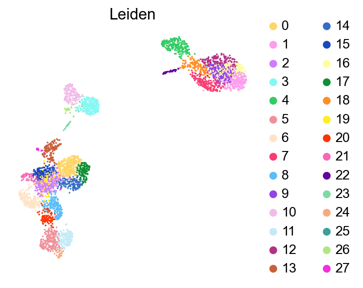
sc.pl.umap(adata,
           color=['Leiden'],
           palette=piaso.pl.color.d_color20,
           legend_fontsize=12,
           legend_fontoutline=2,
           # legend_loc='on data',
           ncols=1,
           size=10,
           frameon=False)

Checking potential low quality clusters#
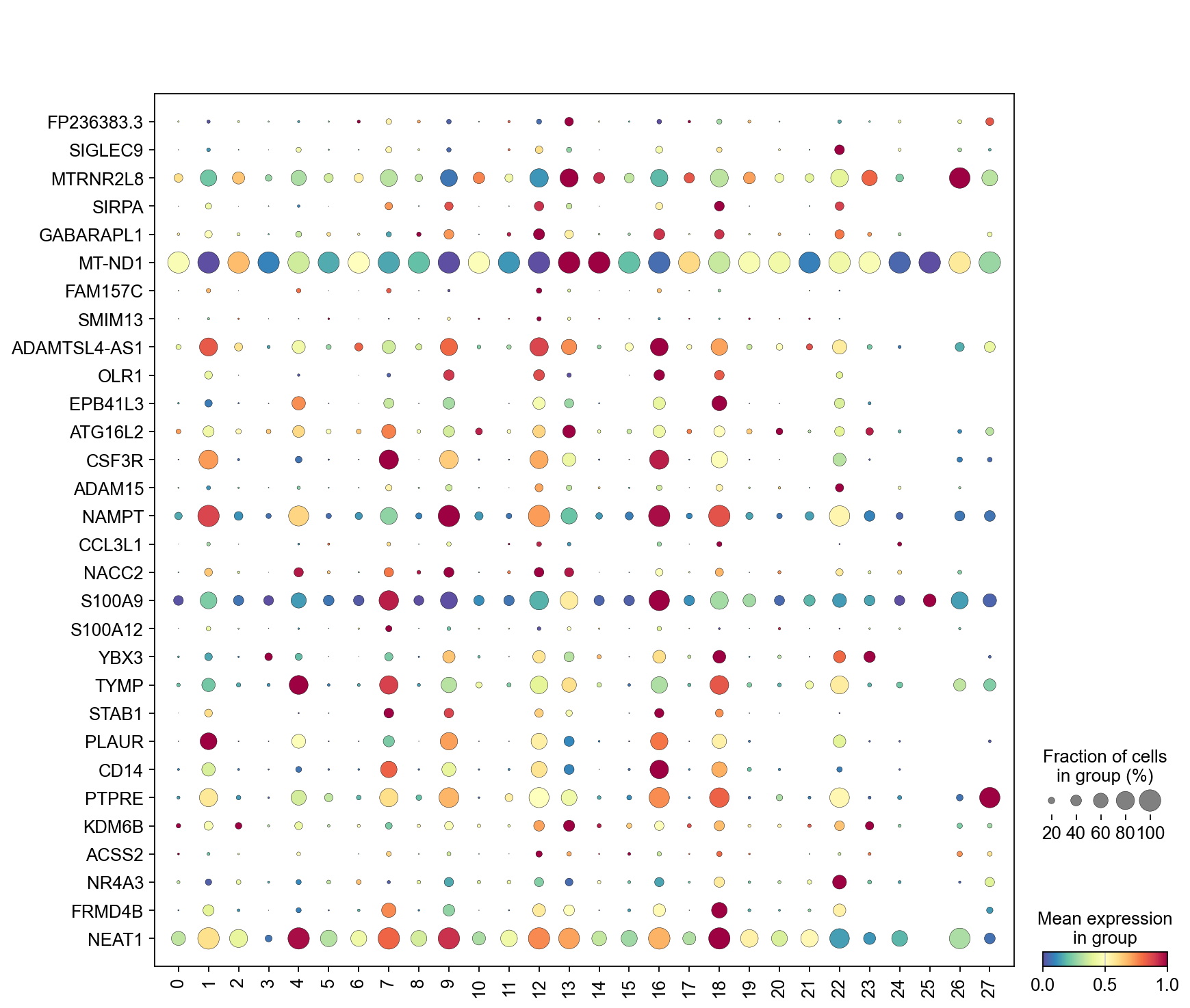
[46]:
cluster_check = '12'
marker_gene[cluster_check].values
[46]:
array(['FP236383.3', 'SIGLEC9', 'MTRNR2L8', 'SIRPA', 'GABARAPL1',
       'MT-ND1', 'FAM157C', 'SMIM13', 'ADAMTSL4-AS1', 'OLR1', 'EPB41L3',
       'ATG16L2', 'CSF3R', 'ADAM15', 'NAMPT', 'CCL3L1', 'NACC2', 'S100A9',
       'S100A12', 'YBX3', 'TYMP', 'STAB1', 'PLAUR', 'CD14', 'PTPRE',
       'KDM6B', 'ACSS2', 'NR4A3', 'FRMD4B', 'NEAT1'], dtype=object)
[47]:
sc.pl.umap(adata,
           color=['FP236383.3', 'SIGLEC9', 'MTRNR2L8', 'SIRPA', 'GABARAPL1',
                  'MT-ND1', 'FAM157C', 'SMIM13', 'ADAMTSL4-AS1', 'OLR1', 'EPB41L3'],
           cmap=piaso.pl.color.c_color1,
           palette=piaso.pl.color.d_color1,
           ncols=3,
           size=10,
           frameon=False)
[48]:
sc.pl.dotplot(adata,
              marker_gene[cluster_check].values[:30],
              groupby='Leiden',
              dendrogram=False,
              swap_axes=True,
              standard_scale='var',
              cmap='Spectral_r')
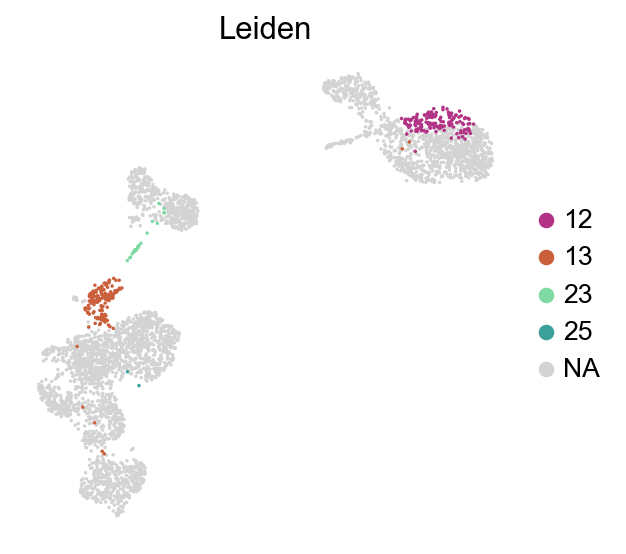
[49]:
sc.pl.umap(adata,
           color=['Leiden'],
           groups=['12','13','23','25'],
           palette=piaso.pl.color.d_color20,
           legend_fontsize=12,
           legend_fontoutline=2,
           # legend_loc='on data',
           ncols=1,
           size=10,
           frameon=False)

[50]:
adata=adata[~adata.obs['Leiden'].isin(['12','13','23','25'])].copy()
2. INFOG Normalization#
It is important to re-run INFOG normalization and dimensionality reduction after filtering out cells, to accurately capture the current cell population.
[51]:
%%time
piaso.tl.infog(adata,
               copy=False,
               inplace=False,
               n_top_genes=3000,
               key_added='infog',
               key_added_highly_variable_gene='highly_variable',
               layer='raw')
The normalized data is saved as `infog` in `adata.layers`.
The highly variable genes are saved as `highly_variable` in `adata.var`.
Finished INFOG normalization.
CPU times: user 310 ms, sys: 113 ms, total: 422 ms
Wall time: 423 ms
Dimensionality reduction#
[52]:
%%time
piaso.tl.runSVD(adata,
                use_highly_variable=True,
                n_components=30,
                random_state=10,
                key_added='X_svd',
                layer='infog')
CPU times: user 2.08 s, sys: 2.67 ms, total: 2.09 s
Wall time: 366 ms
[53]:
%%time
sc.pp.neighbors(adata,
                use_rep='X_svd',
                n_neighbors=15,
                random_state=10,
                knn=True,
                method="umap")

sc.tl.umap(adata)
CPU times: user 14.3 s, sys: 6.15 ms, total: 14.3 s
Wall time: 11.4 s
Predict cell types based on marker gene sets#
[54]:
%%time
piaso.tl.predictCellTypeByMarker(adata,
                                 marker_gene_set=marker_gene_dict,
                                 score_method='piaso',
                                 use_rep='X_svd',
                                 use_score=False,
                                 key_added = 'CellTypes_predicted',
                                 smooth_prediction=True,
                                 inplace=True)
Calculating gene set scores using piaso method...
Scoring gene sets: 100%|██████████| 29/29 [00:15<00:00, 1.91set/s]
Predicting cell types based on marker gene p-values...
Smoothing cell type predictions...
Smoothing cell type predictions from 'CellTypes_predicted_raw' using 7-nearest neighbors
Smoothed predictions stored in adata.obs['CellTypes_predicted_smoothed']
Confidence scores stored in adata.obs['CellTypes_predicted_smoothed_confidence']
Modified 766 cell labels (22.07% of total)
Cell type prediction completed. Results saved to:
  - adata.obs['CellTypes_predicted']: predicted cell types
  - adata.obsm['CellTypes_predicted_score']: full score matrix
  - adata.obsm['CellTypes_predicted_nlog10pvals']: full -log10(p-value) matrix
  - adata.obs['CellTypes_predicted_nlog10pvals']: maximum -log10(p-values)
  - adata.obs['CellTypes_predicted_raw']: original unsmoothed predictions
  - adata.obs['CellTypes_predicted_confidence_smoothed']: smoothing confidence scores
CPU times: user 3.2 s, sys: 73 ms, total: 3.28 s
Wall time: 19.8 s
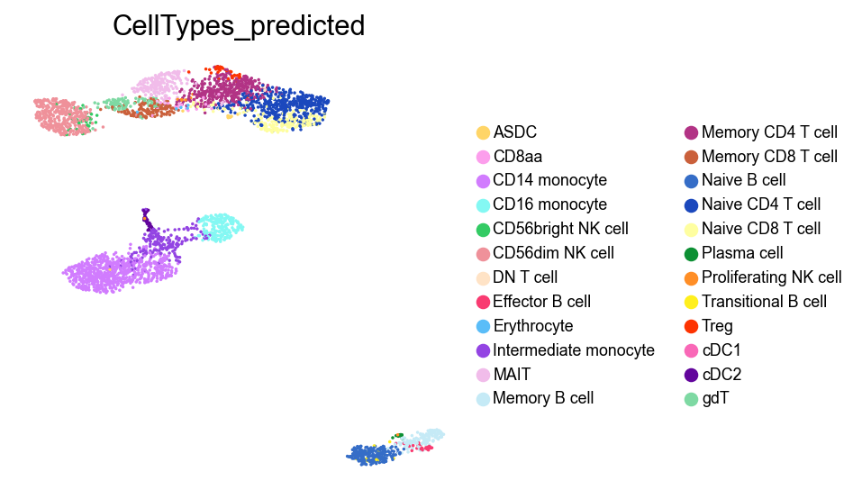
[55]:
sc.pl.umap(adata,
           color=['CellTypes_predicted'],
           palette=piaso.pl.color.d_color20,
           legend_fontsize=8,
           legend_fontoutline=1,
           # legend_loc='on data',
           ncols=1,
           size=10,
           frameon=False)
Identify marker genes with COSG#
[56]:
%%time
n_gene=30
cosg.cosg(adata,
          key_added='cosg',
          use_raw=False,
          layer='infog',
          mu=100,
          expressed_pct=0.1,
          remove_lowly_expressed=True,
          n_genes_user=n_gene,
          groupby='CellTypes_predicted')
CPU times: user 449 ms, sys: 1.99 ms, total: 451 ms
Wall time: 452 ms
[57]:
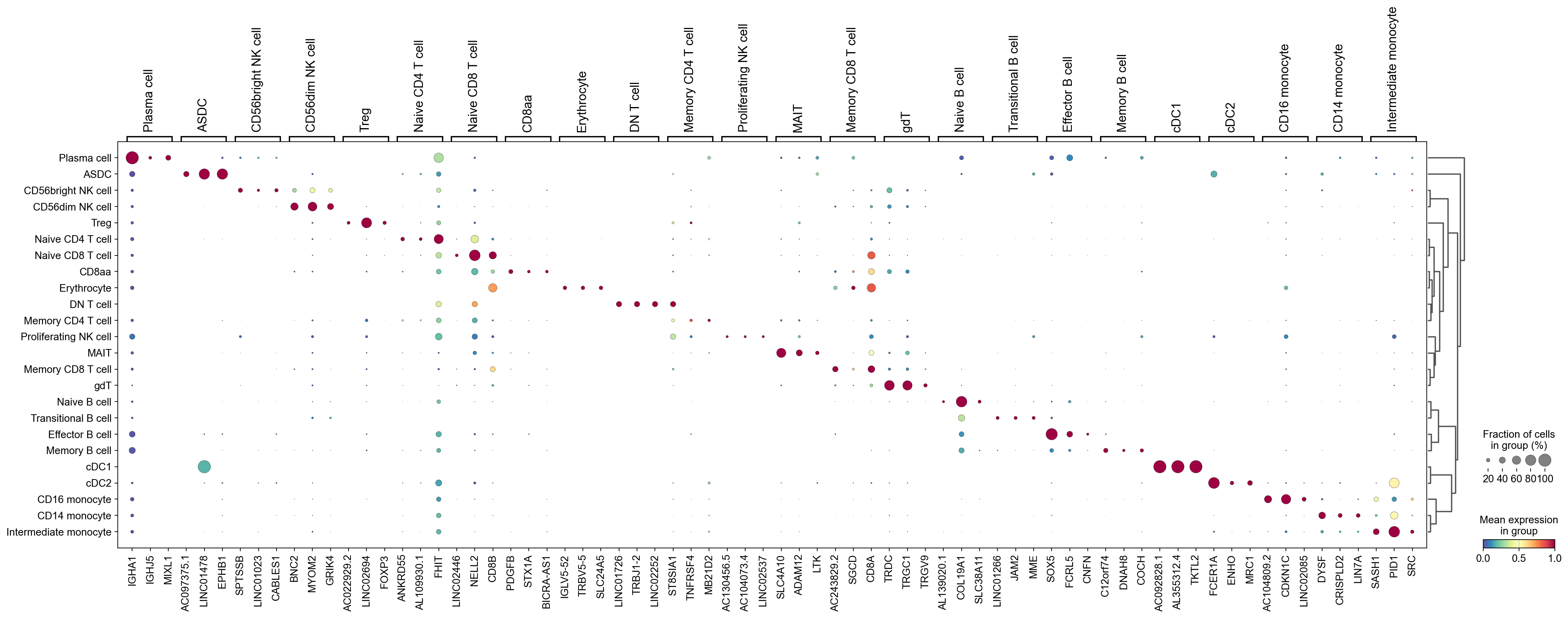
marker_gene=pd.DataFrame(adata.uns['cosg']['names'])
marker_gene
[57]:
| ASDC | CD8aa | CD14 monocyte | CD16 monocyte | CD56bright NK cell | CD56dim NK cell | DN T cell | Effector B cell | Erythrocyte | Intermediate monocyte | ... | Naive B cell | Naive CD4 T cell | Naive CD8 T cell | Plasma cell | Proliferating NK cell | Transitional B cell | Treg | cDC1 | cDC2 | gdT | |
|---|---|---|---|---|---|---|---|---|---|---|---|---|---|---|---|---|---|---|---|---|---|
| 0 | AC097375.1 | PDGFB | DYSF | AC104809.2 | SPTSSB | BNC2 | LINC01726 | SOX5 | IGLV5-52 | SASH1 | ... | AL139020.1 | ANKRD55 | LINC02446 | IGHA1 | AC130456.5 | LINC01266 | AC022929.2 | AC092828.1 | FCER1A | TRDC |
| 1 | LINC01478 | STX1A | CRISPLD2 | CDKN1C | LINC01023 | MYOM2 | TRBJ1-2 | FCRL5 | TRBV5-5 | PID1 | ... | COL19A1 | AL109930.1 | NELL2 | IGHJ5 | AC104073.4 | JAM2 | LINC02694 | AL355312.4 | ENHO | TRGC1 |
| 2 | EPHB1 | BICRA-AS1 | LIN7A | LINC02085 | CABLES1 | GRIK4 | LINC02252 | CNFN | SLC24A5 | SRC | ... | SLC38A11 | FHIT | CD8B | MIXL1 | LINC02537 | MME | FOXP3 | TKTL2 | MRC1 | TRGV9 |
| 3 | LRRC26 | SLC35C1 | VCAN | LYPD2 | TNFRSF11A | SPON2 | OOSP1 | WSCD2 | LONRF2 | CPVL | ... | IGHD | TSHZ2 | NRCAM | JCHAIN | ACRV1 | PYCR3 | FANK1 | HOXA10 | CD1C | KLRC1 |
| 4 | AC018643.1 | MLST8 | PADI4 | GPR20 | XCL1 | LINGO2 | LINC01169 | TLCD4 | CR382287.2 | AC009093.2 | ... | LIX1-AS1 | KANK1 | GLIS3 | SDC1 | AC022517.1 | LINC00494 | AC013652.1 | TACSTD2 | CLEC10A | PTMS |
| 5 | CUX2 | ZSCAN26 | NLRP12 | AC020651.2 | AC002429.2 | MIR181A2HG | AC016727.3 | UQCRHL | LINC00664 | EPB41L3 | ... | AKAP6 | LEF1 | AL590006.1 | IGHV3-15 | AC007179.1 | NEIL1 | HACD1 | AC109347.1 | PKIB | IL12RB2 |
| 6 | AC023590.1 | MAMLD1 | WLS | PPP1R17 | PPP1R9A | CD160 | AC023154.1 | SIGLEC6 | RND2 | IGF2BP2 | ... | PCDH9 | PLCL1 | CA6 | VPREB1 | LINC02289 | AC103831.1 | DUSP4 | ZBTB46-AS1 | LRP1B | CCL5 |
| 7 | KCNK1 | AGMAT | CXCL8 | CKB | ZMAT4 | FGFBP2 | AC026765.3 | PTCHD1-AS | AC023669.2 | RTN1 | ... | LINC00926 | AK5 | LRRN3 | IGKV3-15 | AC005703.7 | AL365272.1 | RTKN2 | ARHGEF3-AS1 | NCKAP5 | AC010175.1 |
| 8 | AC104819.3 | MRPS2 | FCAR | HES4 | SERPINE1 | LDB2 | SLC14A2 | CLECL1 | AC011477.9 | PSAP | ... | LIX1 | EDAR | PDE3B | IGHV3-30 | SNHG18 | TIMP3 | CDHR3 | AC069410.1 | CD1E | S100B |
| 9 | AP000146.1 | AL137779.1 | LUCAT1 | LYNX1 | AL590807.1 | LINC01505 | AC092683.2 | WNT16 | AL133343.2 | IFI30 | ... | ABCB4 | FAM153A | THEMIS | MZB1 | Z92544.2 | STIL | WEE1 | AL356056.1 | ST18 | LINC00612 |
| 10 | AC097375.2 | PPP2R1B | AL163541.1 | CROCC2 | RAMP1 | IGFBP7 | C17orf98 | SLCO4A1 | AC067838.1 | PTGIR | ... | FCER2 | LEF1-AS1 | CACHD1 | ITGA8 | NADK2-AS1 | TCL6 | EVC2 | AC141586.3 | HTR7 | KLRG1 |
| 11 | CYYR1 | AC004918.1 | PRICKLE1 | VMO1 | EFHC2 | LINC00298 | ZNF843 | GALNTL6 | AC114971.1 | CD300E | ... | KHDRBS2 | ITGA6 | SCML1 | GLDC | LINC02721 | AC139795.2 | CCR10 | CLNK | DTNA | A2M |
| 12 | LAMP5 | CRTAM | GLT1D1 | FMNL2 | KLRC2 | MMP23B | AC004223.2 | AC116534.1 | TESC-AS1 | AC020656.1 | ... | STEAP1B | MAN1C1 | APBA2 | TXNDC5 | AC022296.4 | SMIM15 | STAM | CLEC9A | FLT3 | PZP |
| 13 | NRP1 | AC025917.1 | CSF3R | PAPSS2 | NCAM1 | PRF1 | OSGEPL1-AS1 | AL592429.2 | AC003988.1 | MARCO | ... | FCRL1 | CHRM3-AS2 | SNTG2 | TNFRSF17 | PPP1R14B-AS1 | PPAN | FGFR1 | BCHE | SLAMF8 | CACNA2D2 |
| 14 | LINC01724 | CDC14B | VCAN-AS1 | NEURL1 | KLRC3 | PRSS23 | AC008914.1 | TNFRSF13B | AKR1C4 | ZC3H12C | ... | SCN3A | PRKCA | CRTAM | AL357873.1 | AL138759.1 | ZNF486 | GMNN | HLA-DQB1-AS1 | CST3 | TNFSF14 |
| 15 | LINC00865 | STMN3 | NRG1 | SMIM25 | C1orf141 | GZMB | AKR1C1 | LINC02669 | AC134407.1 | LYZ | ... | IL4R | TRABD2A | CD8A | IGLV2-14 | AC002563.1 | AC078980.1 | ZC2HC1A | CLSTN2 | DEPTOR | A2M-AS1 |
| 16 | PHEX | KIF21A | ACSL1 | C1QA | C6orf226 | CLIC3 | AC243965.1 | GPM6A | C20orf144 | LILRB4 | ... | LARGE1 | EPHX2 | LRRC7 | PLAAT2 | SRARP | MAP2 | SNX21 | LRRC49 | HLA-DRB1 | COL6A2 |
| 17 | LINC01226 | AL645728.1 | AQP9 | ICAM4 | TSPAN2 | RHOBTB3 | RAB3C | AL031728.1 | SPACA3 | FADS1 | ... | AFF3 | MAL | EPHA1-AS1 | CNKSR1 | CR381670.2 | AC061958.1 | ICA1 | SMO | ZNF366 | HOPX |
| 18 | TCF4-AS1 | IVD | SPOCK1 | TCF7L2 | TNFRSF18 | AKR1C3 | LINC00536 | AC022509.2 | AC112512.1 | FCGRT | ... | PAX5 | RPL34-AS1 | PRKCA-AS1 | IGLC2 | GRIK1-AS1 | AC098829.1 | MCF2L2 | MIR924HG | HLA-DPA1 | SH3BGRL3 |
| 19 | PTPRS | GCLM | CYP1B1 | LINC02345 | LINC01146 | KLRF1 | EPPK1 | AC090541.1 | CYB5D1 | FGL2 | ... | AC108879.1 | MLLT3 | PRKAR1B | IGHG2 | FAM215A | C14orf119 | TTN | AC022217.2 | IL1R2 | LINC00987 |
| 20 | PTCRA | MGAT2 | LINC00937 | SFTPD | KLHL23 | PDGFD | AL591684.1 | SYT1 | GRIA3 | EMILIN2 | ... | SYN3 | IL6ST | AC009041.2 | GPRC5D | S100A2 | ZNF350-AS1 | OSBP2 | AC104964.1 | CLIC2 | GNLY |
| 21 | LILRA4 | SMYD2 | PLBD1 | CEACAM3 | XCL2 | TTC38 | BNIPL | AC109446.3 | SPDYE2B | MRAS | ... | AC120193.1 | AL163932.1 | NR3C2 | IGKC | DUSP13 | CD180 | IL2RA | LINC01134 | HLA-DPB1 | TGFBR3 |
| 22 | ARPP21 | PBDC1 | TREM1 | KNDC1 | ROR1 | NCR1 | IGSF22 | WDR11-AS1 | AC005498.2 | SECTM1 | ... | ADAM28 | CCR7 | LEF1 | IGLV2-11 | AL138976.2 | ZNF669 | SPSB1 | SHC3 | ITGB5 | LYSMD2 |
| 23 | TDRD1 | C7orf26 | CD36 | LST1 | IL12RB2 | SH2D1B | GINS2 | GEN1 | MOBP | TSPAN4 | ... | KCNH8 | CAMK4 | ABLIM1 | KCNMA1 | AP005209.2 | FAM3C | IKZF2 | KCND3 | NEGR1 | GZMM |
| 24 | PLCB4 | CORO2A | LPAR1 | MS4A7 | ATP8B4 | SORBS2 | AL033528.2 | MS4A1 | ZSCAN23 | LGALS3 | ... | IGHM | IGF1R | CCR7 | AC009570.2 | TROAP | ADGRF3 | MIAT | LAMB2 | ADGRG6 | C1orf21 |
| 25 | SLC35F3 | NIPSNAP3A | RBM47 | SIGLEC10 | GPR68 | RNF165 | LINC01949 | PLPP3 | LINC01182 | CFP | ... | SLC9A7 | OXNAD1 | PSMA1 | EML6 | LINC02354 | MIR762HG | ZNF365 | STEAP3 | ZBTB46 | ZDHHC12 |
| 26 | NTM | SAP30L | TNFAIP6 | CLEC4F | IL18R1 | CCL4 | PRMT6 | GRAPL | VWCE | TTYH3 | ... | GLYATL1 | SERINC5 | OXNAD1 | IGHG3 | USP6 | HAUS3 | AC110611.1 | TMEM201 | FZD2 | SH2D1A |
| 27 | COL24A1 | CDKL3 | FAM198B-AS1 | FCGR3A | KLRC1 | S1PR5 | AC093227.1 | EFNA4 | PLEKHA4 | TNFAIP2 | ... | LINC01800 | RNF157 | MAML2 | IGHA2 | PTPN3 | OXSM | CTLA4 | DZIP1L | CYP2S1 | NDUFS3 |
| 28 | AR | AC112722.1 | AC020916.1 | CTSL | KXD1 | IL2RB | AC015911.6 | AC025569.1 | AC074366.1 | NHSL1 | ... | AC019197.1 | PRKCQ-AS1 | NDFIP1 | IGF1 | AC091153.3 | NCAM2 | AK6 | ENOX1 | HLA-DRA | DUSP2 |
| 29 | COL26A1 | SEC23IP | AL034397.3 | SPRED1 | LINC01684 | ANKRD20A4 | PMP22 | CD70 | P3H3 | CTSH | ... | AP001636.3 | TCF7 | ACTN1 | TSHR | TRAV18 | AHCYL1 | TOX | AC092794.1 | LHFPL6 | GZMH |
30 rows × 24 columns
We can use a dendrogram dot plot to visualize the expression of the top three marker genes of each predicted cell type.
[58]:
sc.tl.dendrogram(adata,groupby='CellTypes_predicted',use_rep='X_svd')
df_tmp=pd.DataFrame(adata.uns['cosg']['names'][:3,]).T
df_tmp=df_tmp.reindex(adata.uns['dendrogram_'+'CellTypes_predicted']['categories_ordered'])
marker_genes_list={idx: list(row.values) for idx, row in df_tmp.iterrows()}
marker_genes_list = {k: v for k, v in marker_genes_list.items() if not any(isinstance(x, float) for x in v)}

sc.pl.dotplot(adata,
              marker_genes_list,
              groupby='CellTypes_predicted',
              layer='infog',
              dendrogram=True,
              swap_axes=False,
              standard_scale='var',
              cmap='Spectral_r')
Marker genes for CD16 monocyte#
[59]:
cluster_check = 'CD16 monocyte'
marker_gene[cluster_check].values
[59]:
array(['AC104809.2', 'CDKN1C', 'LINC02085', 'LYPD2', 'GPR20',
       'AC020651.2', 'PPP1R17', 'CKB', 'HES4', 'LYNX1', 'CROCC2', 'VMO1',
       'FMNL2', 'PAPSS2', 'NEURL1', 'SMIM25', 'C1QA', 'ICAM4', 'TCF7L2',
       'LINC02345', 'SFTPD', 'CEACAM3', 'KNDC1', 'LST1', 'MS4A7',
       'SIGLEC10', 'CLEC4F', 'FCGR3A', 'CTSL', 'SPRED1'], dtype=object)
[60]:
sc.pl.umap(adata,
           color=['AC104809.2', 'GPR20', 'CDKN1C', 'AC020651.2', 'C1QA', 'LINC02085',
                  'LYPD2', 'PPP1R17', 'CKB', 'HES4', 'CROCC2', 'FMNL2', 'VMO1'],
           cmap=piaso.pl.color.c_color1,
           palette=piaso.pl.color.d_color1,
           ncols=3,
           size=10,
           frameon=False)
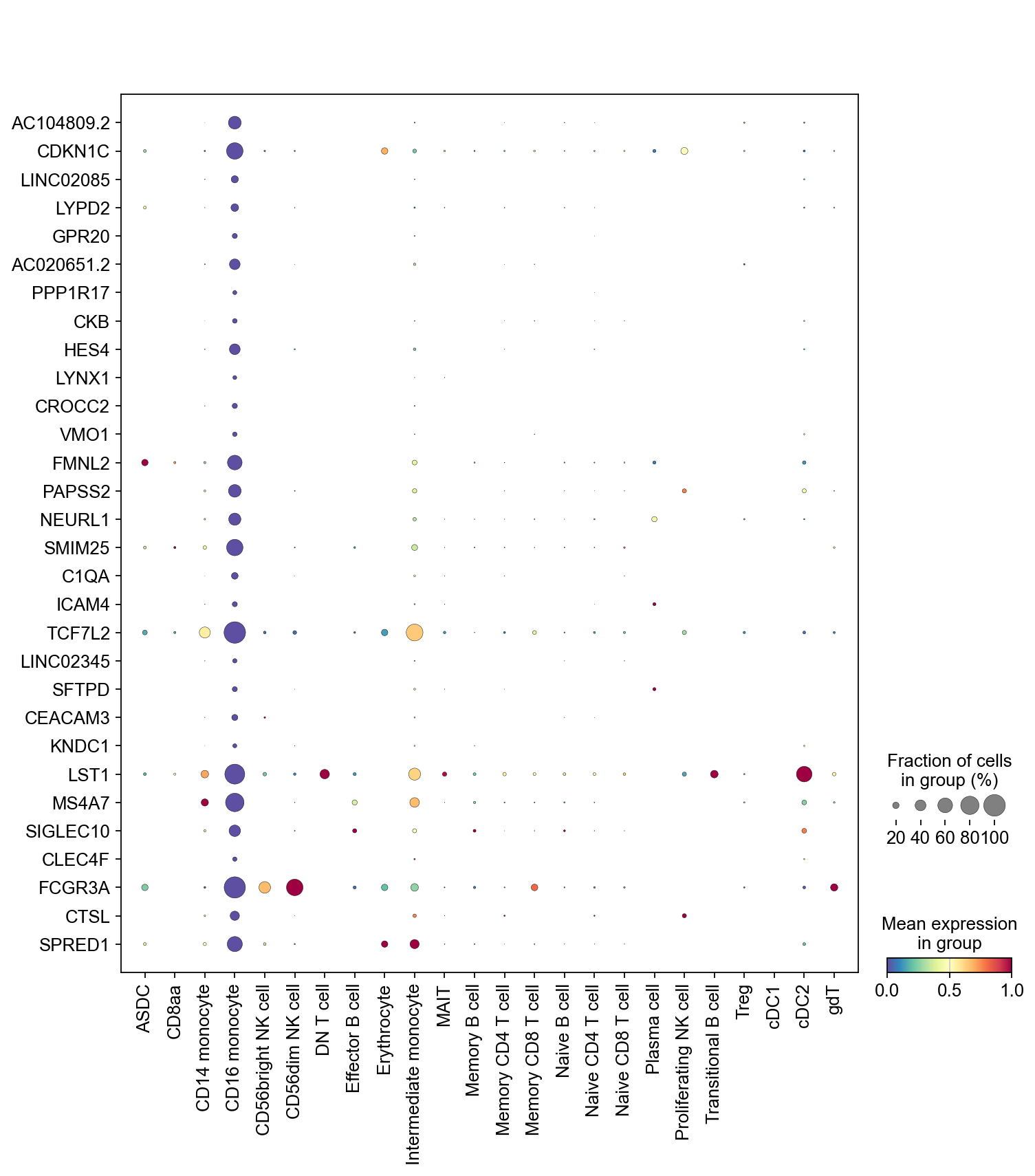
[61]:
sc.pl.dotplot(adata,
              marker_gene[cluster_check].values[:30],
              groupby='CellTypes_predicted',
              dendrogram=False,
              swap_axes=True,
              standard_scale='var',
              cmap='Spectral_r')

Save the data#
[62]:
np.unique(adata.obs['CellTypes_predicted'])
[62]:
array(['ASDC', 'CD14 monocyte', 'CD16 monocyte', 'CD56bright NK cell',
       'CD56dim NK cell', 'CD8aa', 'DN T cell', 'Effector B cell',
       'Erythrocyte', 'Intermediate monocyte', 'MAIT', 'Memory B cell',
       'Memory CD4 T cell', 'Memory CD8 T cell', 'Naive B cell',
       'Naive CD4 T cell', 'Naive CD8 T cell', 'Plasma cell',
       'Proliferating NK cell', 'Transitional B cell', 'Treg', 'cDC1',
       'cDC2', 'gdT'], dtype=object)
[63]:
adata.obs['Sample'] = 0
[64]:
adata.write(save_dir + '/' + prefix + '_QC.h5ad')
[65]:
marker_gene.to_csv(save_dir + '/' + prefix + 'CellType_markerGenes.csv')
[66]:
# adata = sc.read(save_dir + '/' + prefix + '_QC.h5ad')
# adata
[ ]: