Running GDR on MNIST image data#

[1]:

path = '/home/mid166/Analysis/Jupyter/Python/Package/PIASO_github'
import sys
sys.path.append(path)
import piaso

/n/data1/hms/neurobio/fishell/mindai/.conda/envs/scda5/lib/python3.10/site-packages/tqdm/auto.py:21: TqdmWarning: IProgress not found. Please update jupyter and ipywidgets. See https://ipywidgets.readthedocs.io/en/stable/user_install.html
  from .autonotebook import tqdm as notebook_tqdm

[2]:

import scanpy as sc

[3]:

import pandas as pd
import numpy as np

[4]:

sc.set_figure_params(dpi=80,dpi_save=300, color_map='viridis',facecolor='white')
from matplotlib import rcParams
rcParams['figure.figsize'] = 4, 4
save_dir='/n/data1/hms/neurobio/fishell/mindai/Result/single-cell/Methods/Emergene'
sc.settings.figdir = save_dir
prefix='GitHub_testing'

Load the MNIST dataset#

[5]:

from sklearn.datasets import fetch_openml

[6]:

mnist = fetch_openml("mnist_784", version=1)

[7]:

mnist.data

[7]:

	pixel1	pixel2	pixel3	pixel4	pixel5	pixel6	pixel7	pixel8	pixel9	pixel10	...	pixel775	pixel776	pixel777	pixel778	pixel779	pixel780	pixel781	pixel782	pixel783	pixel784
0	0	0	0	0	0	0	0	0	0	0	...	0	0	0	0	0	0	0	0	0	0
1	0	0	0	0	0	0	0	0	0	0	...	0	0	0	0	0	0	0	0	0	0
2	0	0	0	0	0	0	0	0	0	0	...	0	0	0	0	0	0	0	0	0	0
3	0	0	0	0	0	0	0	0	0	0	...	0	0	0	0	0	0	0	0	0	0
4	0	0	0	0	0	0	0	0	0	0	...	0	0	0	0	0	0	0	0	0	0
...	...	...	...	...	...	...	...	...	...	...	...	...	...	...	...	...	...	...	...	...	...
69995	0	0	0	0	0	0	0	0	0	0	...	0	0	0	0	0	0	0	0	0	0
69996	0	0	0	0	0	0	0	0	0	0	...	0	0	0	0	0	0	0	0	0	0
69997	0	0	0	0	0	0	0	0	0	0	...	0	0	0	0	0	0	0	0	0	0
69998	0	0	0	0	0	0	0	0	0	0	...	0	0	0	0	0	0	0	0	0	0
69999	0	0	0	0	0	0	0	0	0	0	...	0	0	0	0	0	0	0	0	0	0

70000 rows × 784 columns

[8]:

mnist.target

[8]:

0        5
1        0
2        4
3        1
4        9
        ..
69995    2
69996    3
69997    4
69998    5
69999    6
Name: class, Length: 70000, dtype: category
Categories (10, object): ['0', '1', '2', '3', ..., '6', '7', '8', '9']

[9]:

adata=sc.AnnData(mnist.data)

/n/data1/hms/neurobio/fishell/mindai/.conda/envs/scda5/lib/python3.10/site-packages/anndata/_core/aligned_df.py:68: ImplicitModificationWarning: Transforming to str index.
  warnings.warn("Transforming to str index.", ImplicitModificationWarning)

[10]:

adata.obs.head()

[10]:


0
1
2
3
4

[12]:

from scipy import sparse

[13]:

adata.X=sparse.csr_matrix(adata.X)

INFOG Normalization#

[14]:

adata.layers['raw']=adata.X.copy()

[15]:

%%time
piaso.tl.infog(adata, layer='raw', n_top_genes=100)

The normalized data is saved as `infog` in `adata.layers`.
The highly variable genes are saved as `highly_variable` in `adata.var`.
Finished INFOG normalization.
CPU times: user 609 ms, sys: 246 ms, total: 855 ms
Wall time: 856 ms

Setting use_highly_variable=False is needed for this dataset:

[16]:

%%time
piaso.tl.runGDRParallel(
    adata,
    groupby=None,
    resolution=1,
    n_gene =100,
    mu = 10,
    layer='raw', infog_layer='raw',
    score_layer='raw',
    scoring_method='piaso',

    random_seed=1927,

    use_highly_variable =False,
    n_highly_variable_genes = 200,

    n_svd_dims =10,

    max_workers = 32,
    calculate_score_multiBatch=False,
    verbosity=0
)

The cell embeddings calculated by GDR were saved as `X_gdr` in adata.obsm.
CPU times: user 1min 55s, sys: 984 ms, total: 1min 56s
Wall time: 2min 5s

[17]:

%%time
sc.pp.neighbors(adata,
                use_rep='X_gdr',
               n_neighbors=15,random_state=10,knn=True,
                method="umap")

sc.tl.umap(adata)

computing neighbors
    finished: added to `.uns['neighbors']`
    `.obsp['distances']`, distances for each pair of neighbors
    `.obsp['connectivities']`, weighted adjacency matrix (0:00:06)
computing UMAP
    finished: added
    'X_umap', UMAP coordinates (adata.obsm)
    'umap', UMAP parameters (adata.uns) (0:00:32)
CPU times: user 50 s, sys: 161 ms, total: 50.1 s
Wall time: 39.2 s

[18]:

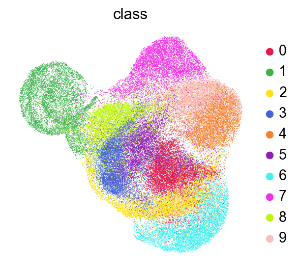
adata.obs['class']=mnist.target.values

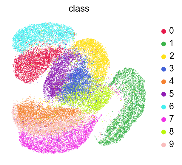
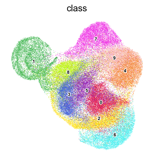
[19]:

sc.pl.umap(adata,
           color=['class'],
           # layer='raw',
           palette=piaso.pl.color.d_color1,
           # cmap=pos_cmap,
           ncols=3,
           # size=10,
           frameon=False)

../_images/notebooks_PIASO_GDR_on_MNIST_21_0.png

[20]:

import matplotlib.pyplot as plt
import numpy as np


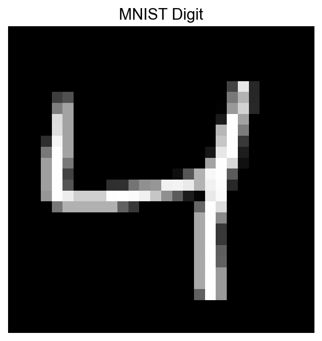
def visualize_mnist_image(image_data):
    # Reshape from 784 pixels to 28x28 image
    image = image_data.reshape(28, 28)

    # Display the image
    plt.figure(figsize=(5, 5))
    plt.imshow(image, cmap='gray')
    plt.axis('off')
    plt.title('MNIST Digit')
    plt.show()

[21]:

visualize_mnist_image(adata[2].X.toarray())

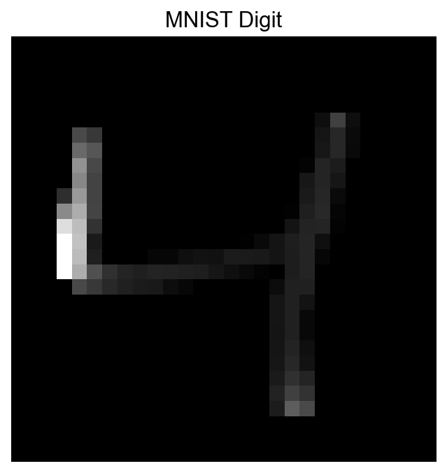
../_images/notebooks_PIASO_GDR_on_MNIST_23_0.png

[22]:

visualize_mnist_image(adata[2].layers['infog'].toarray())

../_images/notebooks_PIASO_GDR_on_MNIST_24_0.png

[23]:

visualize_mnist_image(adata[2].layers['raw'].toarray())

../_images/notebooks_PIASO_GDR_on_MNIST_25_0.png

[24]:

%%time
sc.tl.leiden(adata,resolution=1,key_added='Leiden')

running Leiden clustering

<timed eval>:1: FutureWarning: In the future, the default backend for leiden will be igraph instead of leidenalg.

 To achieve the future defaults please pass: flavor="igraph" and n_iterations=2.  directed must also be False to work with igraph's implementation.

    finished: found 21 clusters and added
    'Leiden', the cluster labels (adata.obs, categorical) (0:01:09)
CPU times: user 1min 9s, sys: 224 ms, total: 1min 9s
Wall time: 1min 9s

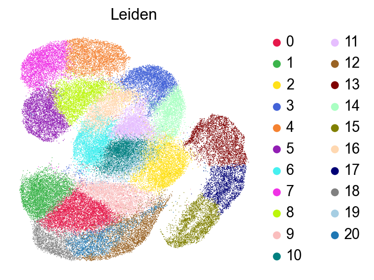
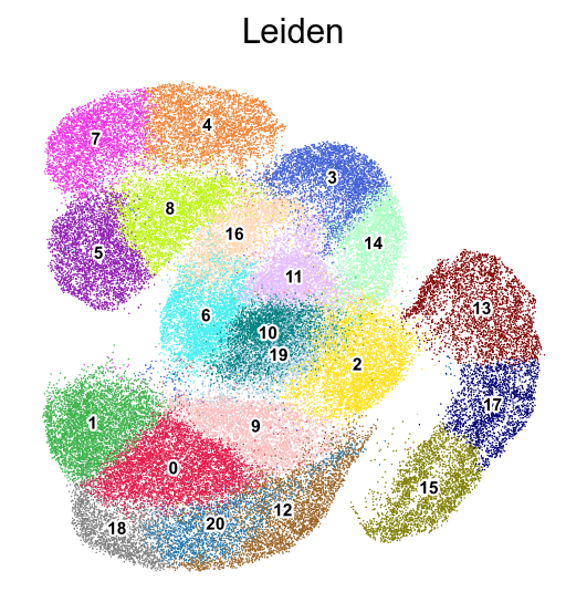
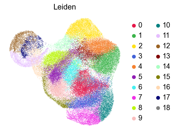
[25]:

sc.pl.umap(adata,
           color=['Leiden'],
           # layer='raw',
           palette=piaso.pl.color.d_color3,
           # cmap=pos_cmap,
           ncols=3,
           # size=10,
           frameon=False)

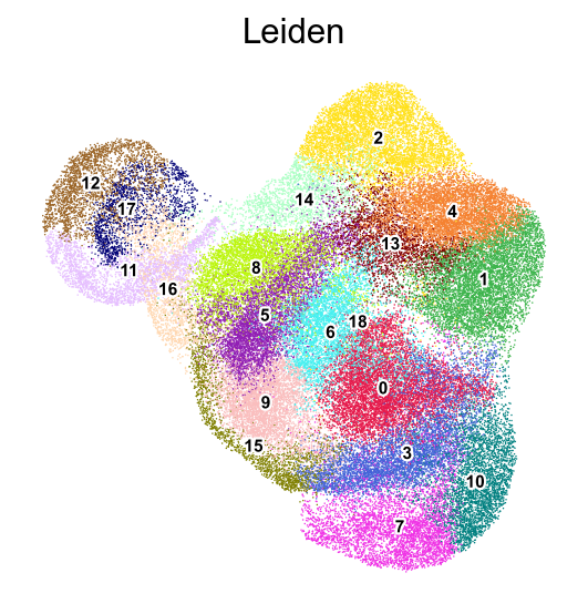
../_images/notebooks_PIASO_GDR_on_MNIST_27_0.png

[26]:

sc.pl.umap(adata,
           color=['Leiden'],
           # layer='raw',
           palette=piaso.pl.color.d_color3,
           legend_fontsize=7,
           legend_fontoutline=2,
           legend_loc='on data',
           # cmap=pos_cmap,
           ncols=3,
           # size=10,
           frameon=False)

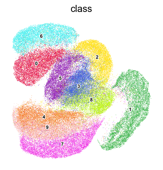
../_images/notebooks_PIASO_GDR_on_MNIST_28_0.png

[ ]:

[27]:

sc.pl.umap(adata,
           color=['class'],
           # layer='raw',
           palette=piaso.pl.color.d_color3,
           legend_fontsize=7,
           legend_fontoutline=2,
           legend_loc='on data',
           # cmap=pos_cmap,
           ncols=3,
           # size=10,
           frameon=False)

../_images/notebooks_PIASO_GDR_on_MNIST_30_0.png

[28]:

def visualize_cluster(X, cluster_labels, cluster_id, num_samples=7):
    # Find all samples belonging to the specified cluster
    indices = np.where(cluster_labels == cluster_id)[0]

    # Select random samples from this cluster (or first few if less than requested)
    sample_indices = indices[:min(num_samples, len(indices))]

    # Create a figure with subplots
    fig, axes = plt.subplots(1, len(sample_indices), figsize=(len(sample_indices)*2, 2))

    # Display each sample
    for i, idx in enumerate(sample_indices):
        ax = axes[i] if len(sample_indices) > 1 else axes
        ax.imshow(X[idx].reshape(28, 28), cmap='gray')
        ax.set_title(f'Cluster {cluster_id}')
        ax.axis('off')

    plt.tight_layout()
    plt.show()

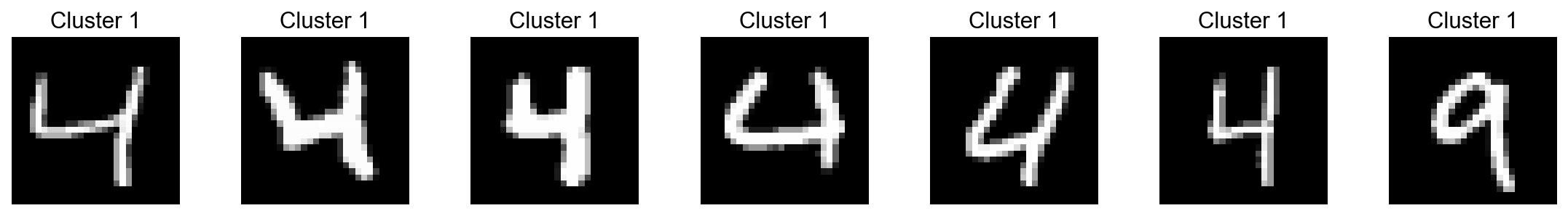
[34]:

visualize_cluster(adata.X.todense(),
                  cluster_labels=adata.obs['Leiden'],
                  cluster_id='1',
                 num_samples=7)

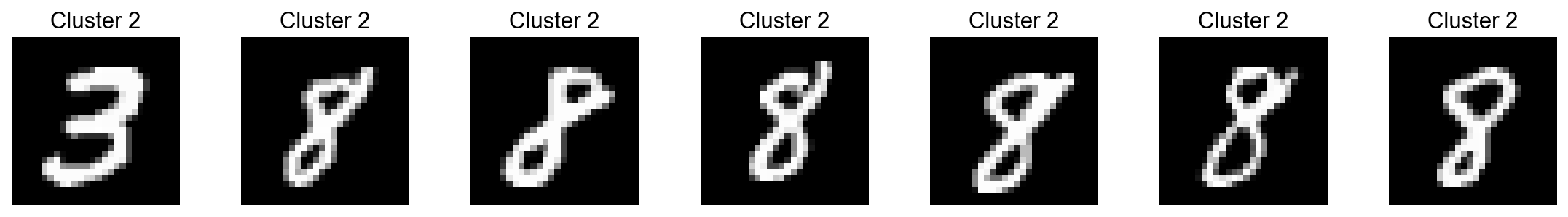
../_images/notebooks_PIASO_GDR_on_MNIST_32_0.png

[35]:

visualize_cluster(adata.X.todense(),
                  cluster_labels=adata.obs['Leiden'],
                  cluster_id='2')

../_images/notebooks_PIASO_GDR_on_MNIST_33_0.png

[36]:

visualize_cluster(adata.X.todense(),
                  cluster_labels=adata.obs['Leiden'],
                  cluster_id='4')

../_images/notebooks_PIASO_GDR_on_MNIST_34_0.png

In a supervised way#

[41]:

%%time
piaso.tl.runGDRParallel(
    adata,
    groupby='class',
    resolution=2.0,
    n_gene =100,
    mu = 10,


    layer='raw', infog_layer='raw',
    score_layer='raw',
    scoring_method='piaso',

    random_seed=1927,


    use_highly_variable =False,
    n_highly_variable_genes = 200,

    n_svd_dims =10,

    max_workers = 32,
    calculate_score_multiBatch=False,
    verbosity=0
)

The cell embeddings calculated by GDR were saved as `X_gdr` in adata.obsm.
CPU times: user 474 ms, sys: 246 ms, total: 720 ms
Wall time: 20.5 s

[42]:

adata.obsm['X_umap_gdr']=adata.obsm['X_umap'].copy()

[43]:

%%time
sc.pp.neighbors(adata,
                use_rep='X_gdr',
               n_neighbors=15,random_state=10,knn=True,
                method="umap")

sc.tl.umap(adata)

computing neighbors
    finished: added to `.uns['neighbors']`
    `.obsp['distances']`, distances for each pair of neighbors
    `.obsp['connectivities']`, weighted adjacency matrix (0:00:06)
computing UMAP
    finished: added
    'X_umap', UMAP coordinates (adata.obsm)
    'umap', UMAP parameters (adata.uns) (0:00:31)
CPU times: user 48.7 s, sys: 113 ms, total: 48.8 s
Wall time: 37.9 s

[44]:

sc.pl.umap(adata,
           color=['class'],
           # layer='raw',
           palette=piaso.pl.color.d_color1,
           # cmap=pos_cmap,
           ncols=3,
           # size=10,
           frameon=False)

../_images/notebooks_PIASO_GDR_on_MNIST_39_0.png

Run Clustering#

[45]:

%%time
sc.tl.leiden(adata,resolution=1,key_added='Leiden')

running Leiden clustering
    finished: found 19 clusters and added
    'Leiden', the cluster labels (adata.obs, categorical) (0:00:58)
CPU times: user 58.3 s, sys: 189 ms, total: 58.4 s
Wall time: 58.6 s

[46]:

sc.pl.umap(adata,
           color=['Leiden'],
           # layer='raw',
           palette=piaso.pl.color.d_color3,
           # cmap=pos_cmap,
           ncols=3,
           # size=10,
           frameon=False)

../_images/notebooks_PIASO_GDR_on_MNIST_42_0.png

[47]:

sc.pl.umap(adata,
           color=['Leiden'],
           # layer='raw',
           palette=piaso.pl.color.d_color3,
           legend_fontsize=7,
           legend_fontoutline=2,
           legend_loc='on data',
           # cmap=pos_cmap,
           ncols=3,
           # size=10,
           frameon=False)

../_images/notebooks_PIASO_GDR_on_MNIST_43_0.png

[48]:

sc.pl.umap(adata,
           color=['class'],
           # layer='raw',
           palette=piaso.pl.color.d_color3,
           legend_fontsize=7,
           legend_fontoutline=2,
           legend_loc='on data',
           # cmap=pos_cmap,
           ncols=3,
           # size=10,
           frameon=False)

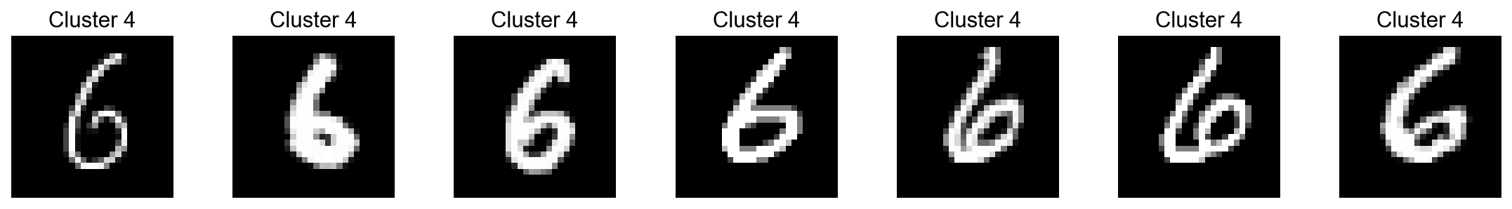
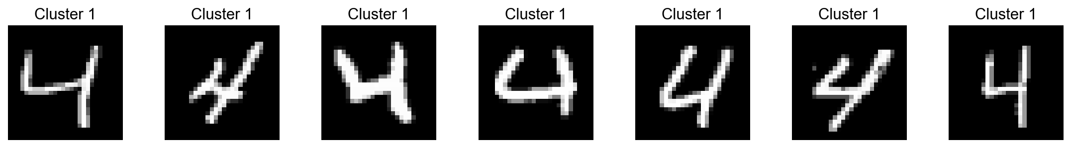
../_images/notebooks_PIASO_GDR_on_MNIST_44_0.png

[50]:

visualize_cluster(adata.X.todense(),
                  cluster_labels=adata.obs['Leiden'],
                  cluster_id='1',
                 num_samples=7)

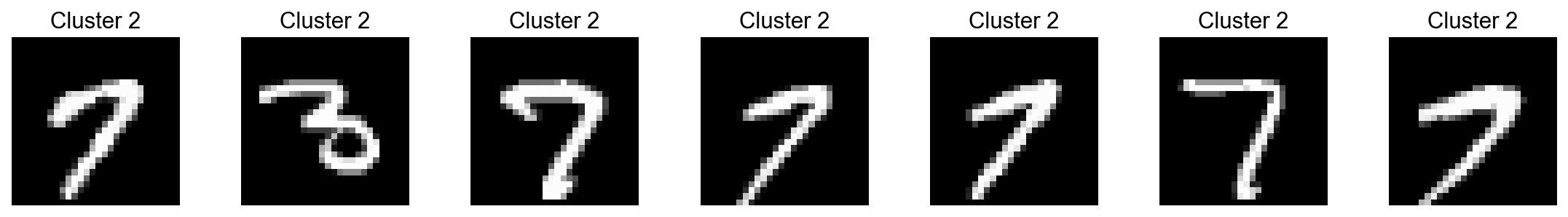
../_images/notebooks_PIASO_GDR_on_MNIST_45_0.png

[51]:

visualize_cluster(adata.X.todense(),
                  cluster_labels=adata.obs['Leiden'],
                  cluster_id='2')

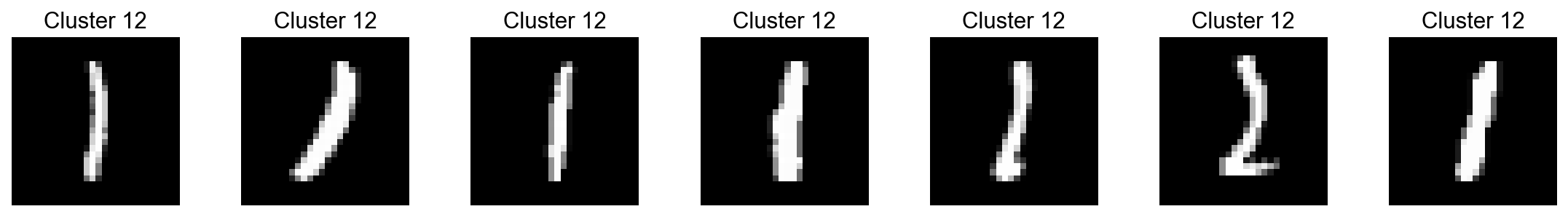
../_images/notebooks_PIASO_GDR_on_MNIST_46_0.png

[53]:

visualize_cluster(adata.X.todense(),
                  cluster_labels=adata.obs['Leiden'],
                  cluster_id='12')

../_images/notebooks_PIASO_GDR_on_MNIST_47_0.png

[ ]: