Finer clustering on selected cluster(s)#
The leiden_local in PIASO is different from using the restrict_to parameter in scanpy’s tl.leiden function, which is running the clustering based on the cell similarity graph built from the whole gene expression matrix containing all the cells. PIASO’s leiden_local function will rerun the dimensional reduction for the selected cluster(s) first and then run the clustering on these cells, so as to better capture the heterogeneity in selected cells.
[1]:
import pandas as pd
import scanpy as sc
import os
from matplotlib import cm
import logging
from matplotlib import rcParams

# To modify the default figure size, use rcParams.
sc.set_figure_params(dpi=80,dpi_save=300, color_map='viridis',facecolor='white')
rcParams['figure.figsize'] = 5, 5
rcParams['font.sans-serif'] = "Arial"
rcParams['font.family'] = "Arial"
sc.settings.verbosity = 3
sc.logging.print_header()
scanpy==1.10.3 anndata==0.10.8 umap==0.5.7 numpy==1.26.4 scipy==1.13.0 pandas==2.2.3 scikit-learn==1.5.2 statsmodels==0.14.4 igraph==0.11.5 louvain==0.8.2 pynndescent==0.5.13
[2]:
path = '/home/vas744/Analysis/Python/Packages/PIASO'
import sys
sys.path.append(path)
import piaso
/home/vas744/.local/lib/python3.9/site-packages/networkx/utils/backends.py:135: RuntimeWarning: networkx backend defined more than once: nx-loopback
  backends.update(_get_backends("networkx.backends"))
Load the data#
We will use the 20k subsampled version of the Seattle Alzheimer’s Disease Brain Cell Atlas (SEA-AD) project dataset described in detail in Gabitto et. al. (2024). We will be using the scRNA-seq data from the dataset in this tutorial. Please refer to the Introduction tutorial to learn more about how it was preprocessed and normalized.
Download the subsampled, pre-processed dataset from Google Drive: https://drive.google.com/file/d/1pDBIgPvEO-sBuIMEhrvVhnf7tfU7H6Xy/view?usp=drive_link
The original data is available on https://portal.brain-map.org/explore/seattle-alzheimers-disease
[3]:
data_dir = "/n/scratch/users/v/vas744/Data/Public/PIASO"
[ ]:
!/home/vas744/Software/gdrive files download --overwrite --destination {data_dir} 1pDBIgPvEO-sBuIMEhrvVhnf7tfU7H6Xy
[5]:
adata=sc.read(data_dir+ '/SEA-AD_RNA_MTG_subsample_excludeReference_20k_piaso_preprocessed.h5ad')
adata
[5]:
AnnData object with n_obs × n_vars = 20000 × 36601
    obs: 'sample_id', 'Neurotypical reference', 'Donor ID', 'Organism', 'Brain Region', 'Sex', 'Gender', 'Age at Death', 'Race (choice=White)', 'Race (choice=Black/ African American)', 'Race (choice=Asian)', 'Race (choice=American Indian/ Alaska Native)', 'Race (choice=Native Hawaiian or Pacific Islander)', 'Race (choice=Unknown or unreported)', 'Race (choice=Other)', 'specify other race', 'Hispanic/Latino', 'Highest level of education', 'Years of education', 'PMI', 'Fresh Brain Weight', 'Brain pH', 'Overall AD neuropathological Change', 'Thal', 'Braak', 'CERAD score', 'Overall CAA Score', 'Highest Lewy Body Disease', 'Total Microinfarcts (not observed grossly)', 'Total microinfarcts in screening sections', 'Atherosclerosis', 'Arteriolosclerosis', 'LATE', 'Cognitive Status', 'Last CASI Score', 'Interval from last CASI in months', 'Last MMSE Score', 'Interval from last MMSE in months', 'Last MOCA Score', 'Interval from last MOCA in months', 'APOE Genotype', 'Primary Study Name', 'Secondary Study Name', 'NeuN positive fraction on FANS', 'RIN', 'cell_prep_type', 'facs_population_plan', 'rna_amplification', 'sample_name', 'sample_quantity_count', 'expc_cell_capture', 'method', 'pcr_cycles', 'percent_cdna_longer_than_400bp', 'rna_amplification_pass_fail', 'amplified_quantity_ng', 'load_name', 'library_prep', 'library_input_ng', 'r1_index', 'avg_size_bp', 'quantification_fmol', 'library_prep_pass_fail', 'exp_component_vendor_name', 'batch_vendor_name', 'experiment_component_failed', 'alignment', 'Genome', 'ar_id', 'bc', 'GEX_Estimated_number_of_cells', 'GEX_number_of_reads', 'GEX_sequencing_saturation', 'GEX_Mean_raw_reads_per_cell', 'GEX_Q30_bases_in_barcode', 'GEX_Q30_bases_in_read_2', 'GEX_Q30_bases_in_UMI', 'GEX_Percent_duplicates', 'GEX_Q30_bases_in_sample_index_i1', 'GEX_Q30_bases_in_sample_index_i2', 'GEX_Reads_with_TSO', 'GEX_Sequenced_read_pairs', 'GEX_Valid_UMIs', 'GEX_Valid_barcodes', 'GEX_Reads_mapped_to_genome', 'GEX_Reads_mapped_confidently_to_genome', 'GEX_Reads_mapped_confidently_to_intergenic_regions', 'GEX_Reads_mapped_confidently_to_intronic_regions', 'GEX_Reads_mapped_confidently_to_exonic_regions', 'GEX_Reads_mapped_confidently_to_transcriptome', 'GEX_Reads_mapped_antisense_to_gene', 'GEX_Fraction_of_transcriptomic_reads_in_cells', 'GEX_Total_genes_detected', 'GEX_Median_UMI_counts_per_cell', 'GEX_Median_genes_per_cell', 'Multiome_Feature_linkages_detected', 'Multiome_Linked_genes', 'Multiome_Linked_peaks', 'ATAC_Confidently_mapped_read_pairs', 'ATAC_Fraction_of_genome_in_peaks', 'ATAC_Fraction_of_high_quality_fragments_in_cells', 'ATAC_Fraction_of_high_quality_fragments_overlapping_TSS', 'ATAC_Fraction_of_high_quality_fragments_overlapping_peaks', 'ATAC_Fraction_of_transposition_events_in_peaks_in_cells', 'ATAC_Mean_raw_read_pairs_per_cell', 'ATAC_Median_high_quality_fragments_per_cell', 'ATAC_Non-nuclear_read_pairs', 'ATAC_Number_of_peaks', 'ATAC_Percent_duplicates', 'ATAC_Q30_bases_in_barcode', 'ATAC_Q30_bases_in_read_1', 'ATAC_Q30_bases_in_read_2', 'ATAC_Q30_bases_in_sample_index_i1', 'ATAC_Sequenced_read_pairs', 'ATAC_TSS_enrichment_score', 'ATAC_Unmapped_read_pairs', 'ATAC_Valid_barcodes', 'Number of mapped reads', 'Number of unmapped reads', 'Number of multimapped reads', 'Number of reads', 'Number of UMIs', 'Genes detected', 'Doublet score', 'Fraction mitochondrial UMIs', 'Used in analysis', 'Class confidence', 'Class', 'Subclass confidence', 'Subclass', 'Supertype confidence', 'Supertype (non-expanded)', 'Supertype', 'Continuous Pseudo-progression Score', 'Severely Affected Donor', 'n_genes', 'n_genes_by_counts', 'total_counts', 'total_counts_mt', 'pct_counts_mt', 'pct_counts_ribo'
    var: 'gene_ids', 'mt', 'n_cells_by_counts', 'mean_counts', 'pct_dropout_by_counts', 'total_counts', 'means', 'variances', 'residual_variances', 'highly_variable_rank', 'highly_variable'
    uns: 'APOE4 Status_colors', 'Braak_colors', 'CERAD score_colors', 'Cognitive Status_colors', 'Great Apes Metadata', 'Highest Lewy Body Disease_colors', 'LATE_colors', 'Overall AD neuropathological Change_colors', 'Sex_colors', 'Subclass_colors', 'Supertype_colors', 'Thal_colors', 'UW Clinical Metadata', 'X_normalization', 'batch_condition', 'default_embedding', 'hvg', 'log1p', 'neighbors', 'title', 'umap'
    obsm: 'X_scVI', 'X_svd', 'X_umap', 'X_umap_backup'
    layers: 'UMIs', 'log1p', 'raw'
    obsp: 'connectivities', 'distances'
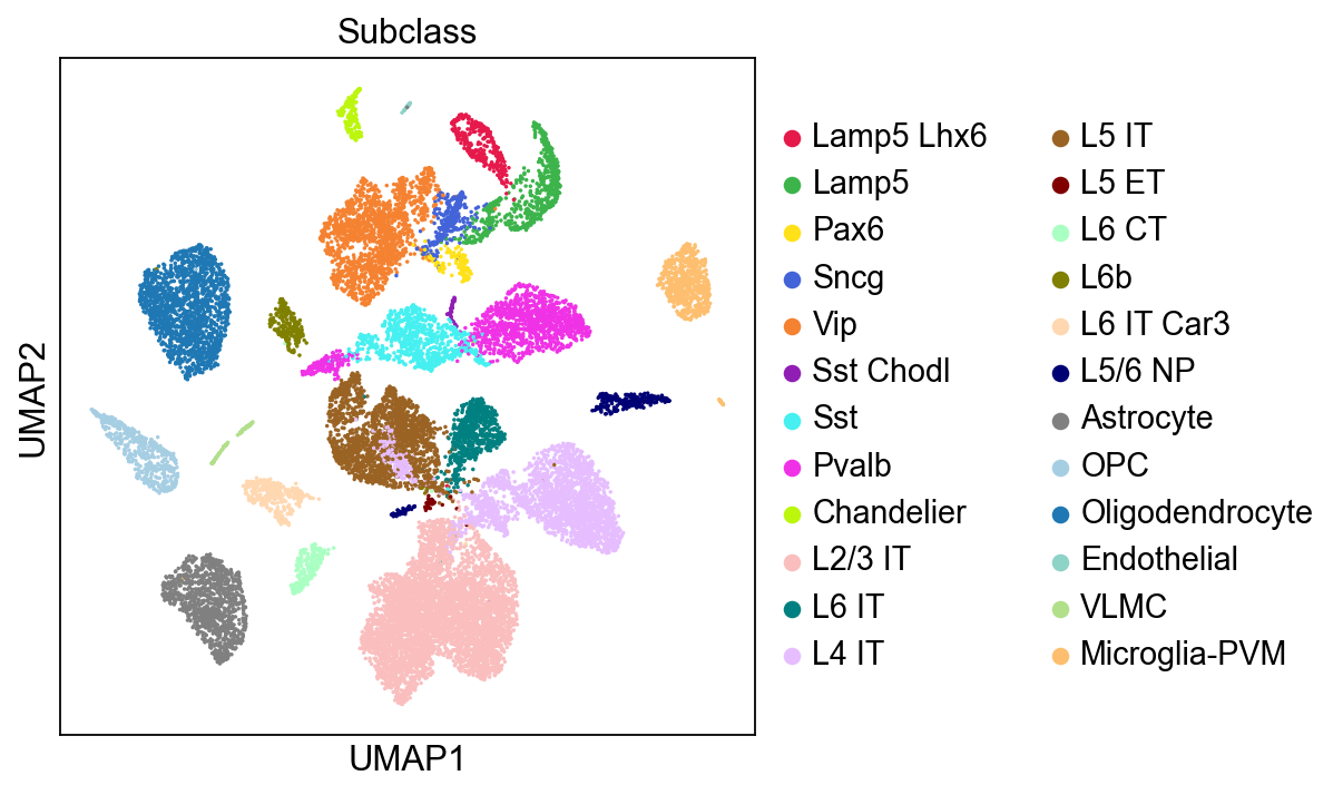
Visualize with UMAP#
[6]:
sc.pl.umap(adata,
           color=['Subclass'],
           palette=piaso.pl.color.d_color4,
           ncols=1,
           size=10,
           frameon=True)
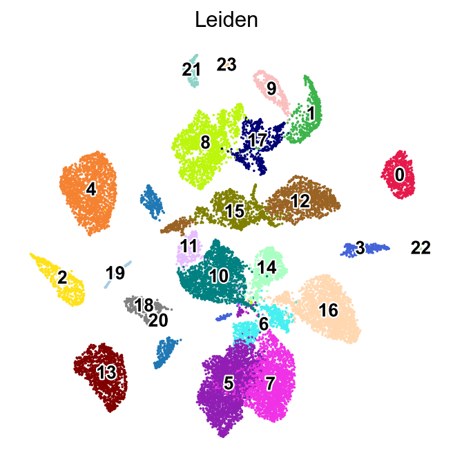
Cluster the data with Leiden algorithm#
[7]:
%%time
sc.tl.leiden(adata,resolution=0.5,key_added='Leiden',flavor="igraph",n_iterations=-1)
running Leiden clustering
    finished: found 24 clusters and added
    'Leiden', the cluster labels (adata.obs, categorical) (0:00:00)
CPU times: user 562 ms, sys: 50.2 ms, total: 612 ms
Wall time: 609 ms
[8]:
logging.getLogger('matplotlib.font_manager').disabled = True
[9]:
sc.pl.umap(adata,
           color=['Leiden'],
           palette=piaso.pl.color.d_color4,
           legend_fontsize=12,
           legend_fontoutline=2,
           legend_loc='on data',
           ncols=1,
           size=10,
           frameon=False)
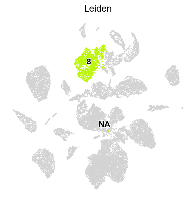
Run leiden_local on one cluster#
Here, we run leiden_local on cluster 8 from the leiden clustering.
[10]:
piaso.tl.leiden_local(adata,
             clustering_type='each',
             groupby='Leiden',
             groups=['8'],
             resolution=0.2,
             batch_key=None,
             key_added='Leiden_local_one',
             dr_method='X_svd_full',
             copy=False)
filtered out 6493 genes that are detected in less than 1 cells
computing neighbors
    finished: added to `.uns['neighbors']`
    `.obsp['distances']`, distances for each pair of neighbors
    `.obsp['connectivities']`, weighted adjacency matrix (0:00:04)
running Leiden clustering
    finished: found 4 clusters and added
    'leiden_local', the cluster labels (adata.obs, categorical) (0:00:00)
/n/data1/hms/neurobio/fishell/vallaris/.conda/envs/genecell_env/lib/python3.9/site-packages/piaso/tools/_clustering.py:191: FutureWarning: In the future, the default backend for leiden will be igraph instead of leidenalg.

 To achieve the future defaults please pass: flavor="igraph" and n_iterations=2.  directed must also be False to work with igraph's implementation.
  sc.tl.leiden(adata_i, resolution=resolution, key_added='leiden_local')
[11]:
sc.pl.umap(adata,
           color=['Leiden'],
           groups=['8'],
           palette=piaso.pl.color.d_color4,
           legend_fontsize=12,
           legend_fontoutline=2,
           legend_loc='on data',
           ncols=1,
           size=10,
           frameon=False)
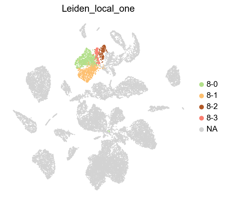
[12]:
sc.pl.umap(adata,
           color=['Leiden_local_one'],
           groups=['8-0','8-1','8-2','8-3'],
           palette=piaso.pl.color.d_color4,
           legend_fontsize=12,
           legend_fontoutline=2,
           ncols=1,
           size=10,
           frameon=False)
Identify markger genes in subclusters#
Identify the marker genes for each sub-cluster identified by leiden local along with all the leiden clusters.
[13]:
import cosg
n_gene=30
cosg.cosg(adata,
          key_added='cosg',
          use_raw=False,
          layer='log1p', ## e.g., if you want to use the log1p layer in adata
          mu=100,
          expressed_pct=0.1,
          remove_lowly_expressed=True,
          n_genes_user=100,
          groupby='Leiden_local_one')
[14]:
sc.tl.dendrogram(adata,groupby='Leiden_local_one',use_rep='X_svd')
df_tmp=pd.DataFrame(adata.uns['cosg']['names'][:3,]).T
df_tmp=df_tmp.reindex(adata.uns['dendrogram_'+'Leiden_local_one']['categories_ordered'])
marker_genes_list={idx: list(row.values) for idx, row in df_tmp.iterrows()}
marker_genes_list = {k: v for k, v in marker_genes_list.items() if not any(isinstance(x, float) for x in v)}

sc.pl.dotplot(adata, marker_genes_list,
              groupby='Leiden_local_one',
              layer='log1p',
              dendrogram=True,
              swap_axes=False,
              standard_scale='var',
              cmap='Spectral_r')
Storing dendrogram info using `.uns['dendrogram_Leiden_local_one']`
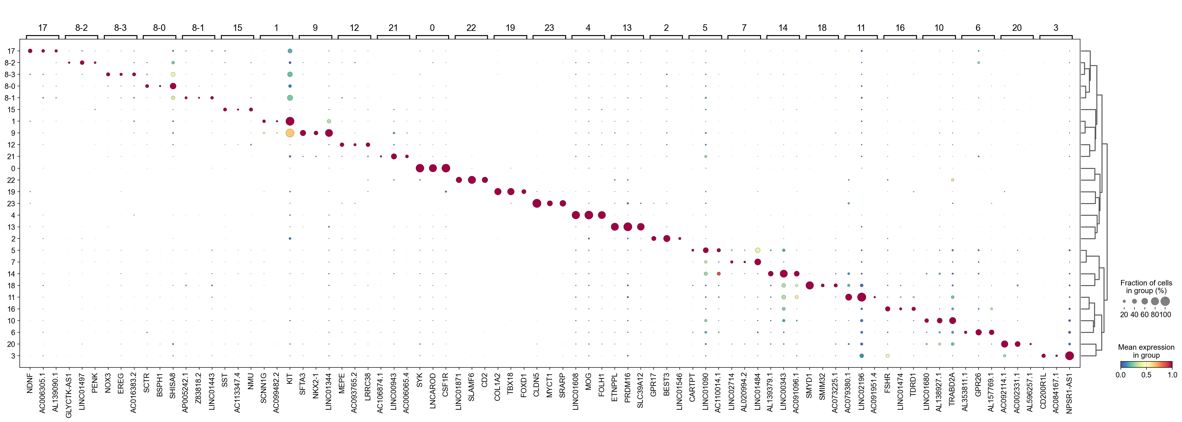
The dotplot reveals that the subclusters identified by leiden_local within leiden cluster 8 exhibit distinct marker genes, suggesting they may differ in nature. Our function successfully detects these differences and can differentiate between the subclusters.
Run leiden_local on multiple clusters#
leiden_local can be run on multiple clusters together, either to identify subclusters within each distinct cluster or identify subclusters across all the given clusters.
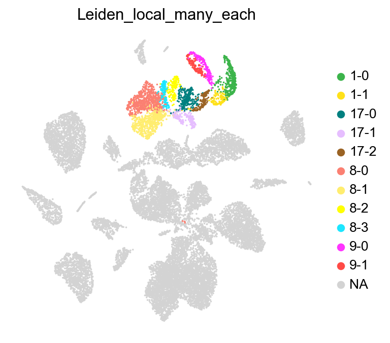
Perform clustering independently within each group#
[15]:
piaso.tl.leiden_local(adata,
             clustering_type='each',
             groupby='Leiden',
             groups=['1','8','9','17'],
             resolution=0.2,
             batch_key=None,
             key_added='Leiden_local_many_each',
             dr_method='X_svd_full',
             copy=False)
filtered out 10206 genes that are detected in less than 1 cells
computing neighbors
    finished: added to `.uns['neighbors']`
    `.obsp['distances']`, distances for each pair of neighbors
    `.obsp['connectivities']`, weighted adjacency matrix (0:00:00)
running Leiden clustering
    finished: found 2 clusters and added
    'leiden_local', the cluster labels (adata.obs, categorical) (0:00:00)
filtered out 6493 genes that are detected in less than 1 cells
computing neighbors
    finished: added to `.uns['neighbors']`
    `.obsp['distances']`, distances for each pair of neighbors
    `.obsp['connectivities']`, weighted adjacency matrix (0:00:00)
running Leiden clustering
    finished: found 4 clusters and added
    'leiden_local', the cluster labels (adata.obs, categorical) (0:00:00)
filtered out 11039 genes that are detected in less than 1 cells
computing neighbors
    finished: added to `.uns['neighbors']`
    `.obsp['distances']`, distances for each pair of neighbors
    `.obsp['connectivities']`, weighted adjacency matrix (0:00:00)
running Leiden clustering
    finished: found 2 clusters and added
    'leiden_local', the cluster labels (adata.obs, categorical) (0:00:00)
filtered out 9092 genes that are detected in less than 1 cells
computing neighbors
    finished: added to `.uns['neighbors']`
    `.obsp['distances']`, distances for each pair of neighbors
    `.obsp['connectivities']`, weighted adjacency matrix (0:00:00)
running Leiden clustering
    finished: found 3 clusters and added
    'leiden_local', the cluster labels (adata.obs, categorical) (0:00:00)
[16]:
sc.pl.umap(adata,
           color=['Leiden_local_many_each'],
           groups=['1-0','1-1','8-0','8-1','8-2','8-3','9-0','9-1','17-0','17-1','17-2'],
           palette=piaso.pl.color.d_color4,
           legend_fontsize=12,
           legend_fontoutline=2,
           ncols=1,
           size=10,
           frameon=False)
Perform clustering across all selected groups#
Here, we will use leiden_local to identify sub-clusters across a group clusters. Let us select a group of subclasses from the data: Lamp5 Lhx6, Lamp5, Pax6, Sncg, and Vip, which are made of clusters ‘1’, ‘8’, ‘9’, and ‘17’.
[17]:
piaso.tl.leiden_local(adata,
             clustering_type='all',
             groupby='Leiden',
             groups=['1','8','9','17'],
             resolution=0.5,
             batch_key=None,
             key_added='Leiden_local_many_all',
             dr_method='X_svd_full',
             copy=False)
filtered out 5168 genes that are detected in less than 1 cells
computing neighbors
    finished: added to `.uns['neighbors']`
    `.obsp['distances']`, distances for each pair of neighbors
    `.obsp['connectivities']`, weighted adjacency matrix (0:00:00)
running Leiden clustering
    finished: found 9 clusters and added
    'leiden_local', the cluster labels (adata.obs, categorical) (0:00:00)
[18]:
sc.pl.umap(adata,
           color=['Leiden_local_many_all'],
           groups=['M-0','M-1','M-2','M-3','M-4','M-5','M-6','M-7','M-8'],
           palette=piaso.pl.color.d_color4,
           legend_fontsize=12,
           legend_fontoutline=2,
           ncols=1,
           size=10,
           frameon=False)
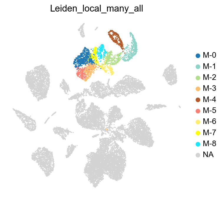
We can compare the subclusters identified by leiden_local with the annotated subclasses from the data, and observe that the identified clusters closely align with the actual subclasses.
[19]:
sc.pl.umap(adata,
           color=['Subclass'],
           palette=piaso.pl.color.d_color4,
           ncols=1,
           size=10,
           frameon=True)
